
The Canadian Seasonal to Interannual Prediction System version 2 (CanSIPSv2)
On this page
- Introduction
- Modifications to models
- Forecast Initialization
- Reforecasts
- Systematic errors
- Skill evaluation of CanSIPSv2 comparing to CanSIPS
- Qualitative evaluation of the parallel run
- Details of implementation
- Summary
- Acknowledgments
- References
- List of Acronyms
1. Introduction
In September 1995 CMC began issuing forecasts for seasonal mean near-surface temperatures and accumulated precipitation in Canada using a two-model ensemble dynamical prediction system based on the first Historical Forecast Project, or HFP (Derome et al. 2001Footnote 1). These forecasts for the standard seasons DJF, MAM, JJA and SON were issued four times per year on December 1, March 1, June 1 and September 1. Initially the two component atmospheric circulation models, each with six ensemble members, were CCCma’s AGCM2 (McFarlane et al. 1992Footnote 2), and the SEF global spectral model developed at Recherche en prévision numérique (RPN; Ritchie, 1991Footnote 3), whereas the GEM model (Côté et al. 1998Footnote 4) developed at RPN replaced the SEF model in March 2004.
CMC began issuing longer-lead statistical forecasts for seasonal mean near-surface temperatures and accumulated precipitation in Canada in late 1996. These forecasts, at lead times of three, six and nine months, were based on application of Canonical Correlation Analysis (CCA) with seasonal means of sea surface temperature (SST) and 500-mb geopotential height over the preceding 12 months as predictors (Shabbar and Barnston 1996Footnote 5). The seasons forecast by this system were the same as the zero-lead dynamical forecasts (except with longer lead) and the dates of issuance were also the same.
The CMC’s dynamical seasonal forecast system underwent a major upgrade in October 2007 to a four-model system using AGCM2, SEF, GEM and CCCma’s AGCM3 (Scinocca et al. 2008Footnote 6) with total of 40 ensemble members, 10 from each model. From the beginning, each 10-member model ensemble was constructed from 24-h lagged initial conditions covering the 10 previous days of the forecast initiation. That period was reduced to 5 days in 2008 by using 12h lags. Seasonal forecasts were issued both at zero-month lead (months 1-3) and one-month lead (months 2-4) on the first day of every month, and a first-month forecast for surface temperature only was issued on the 1st and 15th of every month. Hindcasts for bias correction and skill assessment were provided by the second Historical Forecasting Project (HFP2; Kharin et al. 2009Footnote 7). The CCA-based longer-lead forecasts continued to be issued four times per year.
The main basis for skill in a dynamical seasonal forecasting system is its ability to model the atmospheric response to relatively slowly varying boundary conditions, primarily anomalies in sea surface temperature (SST). Because all the models comprising the HFP and HFP2 systems are atmospheric circulation models with no dynamical ocean, future SSTs in these forecasts had to be prescribed, based on information available at the beginning of the forecast. Although there are numerous possible choices for such a prescription, in the HFP and HFP2 systems SSTs during the forecast periods were specified to be the mean SST anomalies during the 30 days preceding the forecast, added to the seasonally varying SST climatology. Of course, a serious limitation of this prescription of anomaly persistence is that actual SST anomalies evolve with typical time scales of a few months, so that the prescribed SST anomalies at the end of the forecast may not resemble the actual SST anomalies at that time. This limits the utility of such “two-tier” forecast systems beyond forecast periods of a few months, and indeed the HFP forecasts were limited to three months and the HFP2 forecasts to four months for this reason.
The two-tier seasonal forecast system was replaced by the Canadian Seasonal to Interannual Prediction System (CanSIPS) in December 2011, which is a global coupled one-tier system. CanSIPS uses two atmosphere-ocean coupled climate models, CanCM3 and CanCM4, that were developed at CCCma, with a total of 20 ensemble members, 10 from each model. From the beginning of each month, 10 ensemble members of forecast for each model were produced for 12 months from initial conditions of small perturbations at the same time, i.e., with a burst start approach. Details on the CanSIPS system are described in Merryfield et al. (2013)Footnote 8.
It is noteworthy to point out that CanSIPS has been an integral part of several international activities related to multi-model ensemble seasonal forecasts, including the North American Multi-model Ensemble (NMME) (e.g., Kirtman et al. 2014Footnote 9), the WMO Long-Range Forecast Multi-Model Ensemble (e.g., Kim et al. 2015Footnote 10), and the multi-model climate prediction of the Asian-Pacific Economic Cooperation Climate Center (APCC) (e.g., Min, et al. 2014Footnote 11).
From September 1995 to June 2015, output of the first month from the seasonal forecast system was used to produce the 30-day-averaged temperature anomaly forecast, which was the only monthly forecast product in Canada. Since July 2015, the monthly forecast is produced in CMC based on the Global Ensemble Prediction System (GEPS; Gagnon et al. 2015Footnote 12), which takes advantage of the increased resolution and improved initialization of GEPS (Lin et al. 2016Footnote 13)
The most recent update is that the ECCC numerical weather prediction (NWP) model, GEM, is coupled with the NEMO ocean model to develop an NWP-based global atmosphere-ocean-sea ice coupled model, which is called GEM-NEMO. CanCM4 is upgraded to CanCM4i with improved initialization. GEM-NEMO replaces CanCM3 in CanSIPS and is combined with CanCM4i to form the second version of CanSIPS for multi-model ensemble seasonal prediction. Development of GEM-NEMO seasonal forecast model took place mainly at RPN, exploiting the coupled model and modeling expertise available there, which also benefits from the contribution of the CONCEPTS project.
This document describes the latest modifications to the Canadian Seasonal to Interannual Prediction System, becoming CanSIPS version 2, hereafter referred to as CanSIPSv2. In Section 2 we present modifications to the prediction components of CanSIPS in support of the operational implementation of July 2019 to replace CanSIPS. Section 3 describes the forecast initialization. The reforecast is introduced in Section 4. Section 5 describes systematic errors in CanCM2 and GEM-NEMO. Skill evaluation results are presented in Section 6. Section 7 gives evaluation of the parallel run. The detail of implementation is given in Section 8. Finally, we summarize results in Section 9.
The current implementation represents cumulative efforts of many people not only from the CanCM4i and GEM-NEMO teams, but also from other groups such as the modelling and postprocessing sections in research and development divisions, and operational sections of Environment and Climate Change Canada (ECCC) co-located at the Canadian Meteorological Centre (CMC) in Dorval, Québec.
2. Modifications to models
Like its predecessors (the HFP, HFP2, and CanSIPS systems), CanSIPSv2 is a multi-model system which takes advantage of the generally greater skill of multi-model compared to singlemodel systems for a given ensemble size (e.g. Kharin et al. 2009Footnote 7).
CanSIPSv2 consists of two global coupled models, CanCM4i and GEM-NEMO. CanCM4i applies an improved initialization to the same version of the CanCM4 model used previously in CanSIPS. This model is described in detail in Merryfield et al. (2013)Footnote 8, so only its most basic aspects are outlined here. On the other hand, GEM-NEMO is a new model introduced to CanSIPSv2 and will be described in detail here.
2.1 CanCM4i
CanCM4i, like CanCM4, couples CCCma’s fourth-generation atmospheric model CanAM4 to CCCma’s CanOM4 ocean component. Atmospheric horizontal resolution is T63, corresponding to a 128 x 64 Gaussian grid, with 35 vertical levels and a top at 1 hPa. The 256 x 192 grid of CanOM4 provides horizontal resolution of approximately 1.4 degrees in longitude and 0.94 degrees in latitude, with 40 vertical levels. Version 2.7 of the CLASS land surface scheme and a single-category, cavitating-fluid sea ice model are employed, both formulated on the atmospheric model grid.
2.2 GEM-NEMO
GEM-NEMO, developed at the Recherche en Prévision Numérique (RPN), is a fully coupled model with the atmospheric component of GEM (Côté et al. 1998Footnote 4) and the ocean component of NEMO (Nucleus for European Modelling of the Ocean, http://www.nemo-ocean.eu).
The GEM version used is 4.8-LTS.13, with a horizontal resolution of 256 × 128 grid points (about 155 km) evenly spaced on a latitude-longitude grid, and 79 vertical levels with the top at 0.075 hPa. The land scheme is ISBA (Noilhan and Planton, 1989Footnote 14; Noilhan and Mahfouf, 1996Footnote 15), where each grid point is assumed to be independent (no horizontal exchange). The atmospheric deep convection parameterization scheme of Kain-Fritsch (Kain and Fritsch 1990Footnote 16) is used. The Kuotransient scheme (Bélair et al. 2005Footnote 17) is applied for shallow convections. The model allows for vegetation and ozone seasonal evolutions during the integration. The evolution of anthropogenic radiative forcings are treated simply through specification of equivalent CO2 concentrations with a linear trend. The GEM model is integrated with a time step of one hour. Among the 10 ensemble members in both the forecast and the reforecast, implicit surface flux is used in members 1-5 and explicit surface flux is applied in members 6-10.
The ocean model NEMO is NEMO 3.6 ORCA 1 with a horizontal resolution of 1°×1° (1/3 degree meridionally near the equator) and 50 vertical levels. The CICE 4.0 (Community of Ice CodE, Hunke and Lipscomb 2010Footnote 18) model is used for the sea-ice component with five ice categories. The NEMO model is run with a 30-minute time step.
GEM and NEMO are coupled once an hour through the GOSSIP coupler. No flux corrections are employed in the coupled model.
3. Forecast initialization
Similar to what was done in CanSIPS, each of the two models in CanSIPSv2, CanCM4i and GEM-NEMO, makes its real-time forecast once a month, initialized at the beginning of each month. Each model produces forecasts of 10 ensemble members with all the integrations starting from the same date and lasting for 12 months. However, the two models take different approaches in the initialization for the forecasts.
3.1 CanCM4i
The only change in CanCM4i forecast initialization compared to CanCM4 initialization in CanSIPS is that initial conditions for Northern Hemisphere (Arctic) sea ice thickness are obtained from the SMv3 statistical model of Dirkson et al. (2017)Footnote 19. (Additional changes in reforecast initialization that are intended to improve consistency between reforecasts and realtime forecasts are described in section 4.) Other aspects, common to CanCM4 in CanSIPS, are that each CanCM4i ensemble member is initialized from a separate assimilating model run in which atmospheric temperature, moisture, horizontal winds, SST and sea ice concentration are constrained by values from the Global Deterministic Prediction System (GDPS) analysis. Land surface variables are initialized through the response of the land surface component to atmospheric conditions in the assimilating model runs, whereas subsurface ocean temperatures are constrained by values from the Global Ice Ocean Prediction System (GIOPS) analysis through an offline procedure. Details of the initialization methods are provided in Merryfield et al. (2013)Footnote 20.
3.2 GEM-NEMO
In the forecast, the atmospheric initial conditions of GEM-NEMO come from those of the Global Ensemble Prediction System (GEPS; Gagnon et al. 2015Footnote 12), that are generated from EnKF with data assimilation. Ten of the GEPS perturbed initial conditions are used for the GEM-NEMO seasonal forecast.
For the land surface initial conditions, in addition to taking advantage of the CMC analysis one important consideration is to make it consistent with the reforecast. In the reforecast, which will be introduced in section 4.2, we initialize the land surface by running the Surface Prediction System or SPS (Carrera et al. 2010Footnote 21) forced by the near-surface atmospheric and the precipitation fields of the ERA-interim reanalysis. In the real-time forecast, the land surface initial fields are generated by forcing the SPS with the CMC analysis.
The ocean and sea ice initial conditions in the forecast come from the CMC GIOPS analysis (Smith et al. 2016Footnote 22). The near surface air temperature from GEPS and the snow depth from SPS are used for the initialization of these variables over sea ice in CICE. For the reforecast, the ocean and sea ice initial conditions are described in section 4.2. All ensemble members have the same ocean and sea ice initial conditions.
4. Reforecasts
For seasonal predictions, model drift and systematic model errors become a serious problem that contaminates the forecast quality. A common practice in seasonal prediction is to perform a historical reforecast (or hindcast) to estimate the model climatology and statistics, so that calibrated anomaly forecasts can be made. Another purpose of the reforecast is to generate a long record of forecast data to quantify the performance of the forecast system. Therefore, the reforecast is an important component of the seasonal forecast system. As in CanSIPS, the reforecast is made with each individual model, covering 31 years from 1980-2010 with 10 members of 12-month integration starting from the beginning of each month. In the reforecast, each individual model has the same configuration as in the forecast.
4.1 CanCM4i
CanCM4i employs several changes to the CanCM4 reforecast initialization procedure described in Merryfield et al. (2013)Footnote 20. First, as in the real time forecasts, modelled sea ice thickness is constrained near values from the SMv3 statistical model of Dirkson et al. (2017)Footnote 19, which is much more realistic than the stationary model-based climatology employed for CanCM4, in part because it accounts for the long-term thinning of Arctic sea ice. Second, modelled sea ice concentration is constrained near values from the Had2CIS product described in . Had2CIS provides improved temporal consistency across the reforecast period, as well as improved consistency with sea ice concentrations from the GDPS analysis used in real time, compared to the concentration product used to initialize CanCM4 reforecasts. Finally, initial subsurface ocean temperatures are constrained by the ORAP5 ocean reanalysis (Zuo et al. 2015Footnote 23), which is both closer in its formulation to the GIOPS analysis used in real time, and has more realistic trends than the ocean reanalysis used to initialize CanCM4 reforecasts.
4.2 GEM-NEMO
In the reforecast, the atmospheric conditions are initialized using the ERA-interim reanalysis (Dee et al, 2011Footnote 24). Random isotropic perturbations are added to the reanalysis fields to create 10 different initial conditions. The atmospheric perturbations are homogeneous and isotropic as in Gauthier et al. (1999)Footnote 25. Only the streamfunction and the unbalanced temperatures are perturbed as in EnKF (see Houtekamer et al., 2009Footnote 26). These perturbed fields are then transformed to wind, temperature and surface pressure.
The ocean initial fields come from the ORAP5 ocean reanalysis (Zuo et al. 2015Footnote 23). The monthly values of temperature, salinity, zonal and meridional currents are interpolated to daily values. The sea ice concentration initial fields are the Had2CIS, which was prepared by Woo-Sung Lee of CCCma, who combined the digitized sea ice charts from the Canadian Ice Service (CIS) with the HadISST2.2. The original HadISST2.2 employs an ice chart-based bias correction of the passive microwave record (Titchner and Rayner 2014Footnote 27). The monthly HadISST2.2 data, the digitized CIS weekly sea ice charts over the Arctic region and the weekly CIS "Great Lakes ice charts" over Great Lakes are interpolated to daily data before the combination. The sea ice thickness is interpolated from the monthly ORAP5 data. The near surface air temperature from ERA-interim and the snow depth from SPS are used for the initialization of these variables over sea ice in CICE.
For the land surface initialization, we make use of historical dataset of surface fields produced by SPS (Carrera et al. 2010Footnote 21). It is previously known as GEM-surf and it was used in several studies at high resolution (see Separovic et al. 2014Footnote 28, Ioannidou et al. 2014Footnote 29 and Bernier and Bélair 2012Footnote 30). To generate more realistic land surface conditions, we have run the SPS for the period 1980-2010 to create surface fields compatible with the surface scheme of the model. The SPS is simply the surface schemes (land, sea ice and glacier) of the GEM model used in offline mode. To initialize the land surface fields in the reforecast, we have forced SPS by the near-surface atmospheric and the precipitation fields coming from the ERA-interim reanalyses. The surface pressure, the 2-m temperature and dew-point depression as well as the solar and infra-red downward radiative fluxes at the surface are provided to SPS at a 3-hour interval. To limit the snow accumulation over glaciers, the maximum snow depth is set to 12 meters in the initial condition.
5. Systematic Errors
In this section, the systematic error is analyzed for the CanCM4i and GEM-NEMO models, which is the difference between the predicted and observed climatology over the reforecast period of 1981-2010. The objective is to demonstrate the general behavior of the two models related to model drift. When doing seasonal prediction, forecasts of anomalies are produced, where the model climate estimated from the reforecast is subtracted, and the systematic error is removed in the forecast. It thus appears that there is no direct impact of the systematic error on the forecast skill, which will be presented in the next section. However, the systematic error does affect the forecast skill through the model dynamics. For example, a biased middle-latitude westerly jet would lead to errors in Rossby wave propagation and teleconnection patterns forced by ENSO, resulting in an inaccurate anomaly forecast. Therefore, it is important to reduce the model bias.
The verification data are the ERA-interim reanalyses for 2-meter air temperature (T2m) and 200hPa zonal wind (U200), the Global Precipitation Climatology Project (GPCP; Huffman et al. 2009Footnote 31) dataset for precipitation, and the NOAA Optimum Interpolation (OI) Sea Surface Temperature V2 (Reynolds et al. 2002Footnote 32) for SST. The systematic error presented here is for the one-month lead seasonal mean, averaged over the 12 initialization months.
We first look at the model bias of SST, which is shown in Figure 1. As can be seen, CanCM4i is doing a good job in controlling the model drift, with biases only in limited areas near the west coast of South America, east coast of East Asia and North America, and along the tropical Pacific and high latitude North Atlantic and Southern oceans (Figure 1a). On the other hand, GEM-NEMO systematically has cold biases in the tropical oceans (Figure 1b), indicating that the model drift in GEM-NEMO is relatively strong. This is an area of future improvement for GEMNEMO.
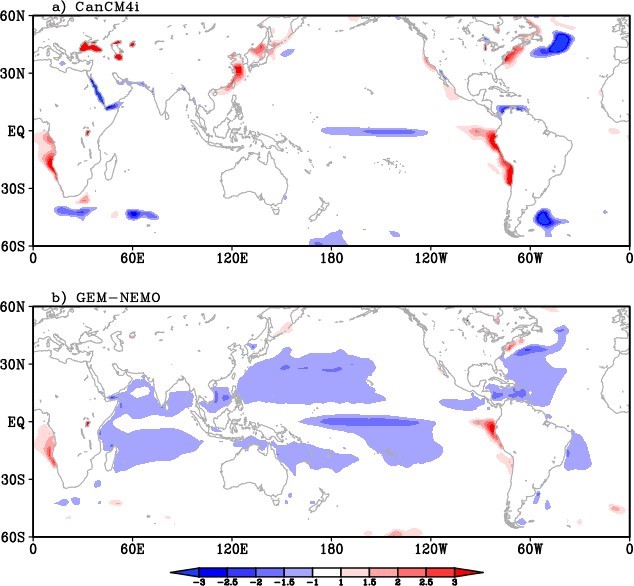
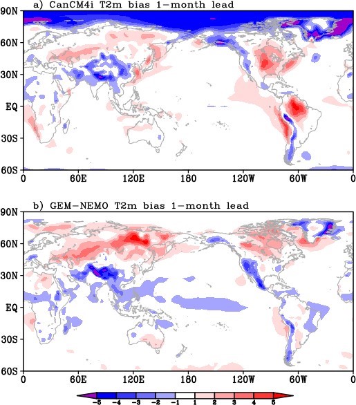
Figure 2 shows the geographical distribution of systematic error for T2m. The CanCM4i model is seen to have quite strong cold biases over the Northern Hemisphere Polar Region (Figure 2a), that may be related to the treatment of sea ice physics, or atmospheric physics over sea ice. Both models have warm T2m biases over the Northern middle-high latitude continents, and cold biases over the mountains. CanCM4i has warm biases over equatorial South America. Over the ocean, CanCM4i shows some warm biases near the west coast of South America, east coast of East Asia and North America. Cold biases are observed in GEM-NEMO in the tropical Pacific, which are related to the SST biases as discussed above.
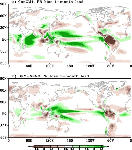
Shown in Figure 3 is the systematic error in precipitation rate. The two models seem to have a similar precipitation bias distribution. Excessive precipitation is found over a large area of the tropics with insufficient precipitation over the equatorial Pacific, a feature of the double– intertropical convergence zone (ITCZ) which is common to many coupled general circulation models (e.g., Lin 2007Footnote 33). The magnitude of the wet bias in CanCM4i is stronger than GEMNEMO. CanCM4i also has a strong wet bias in the tropical Indian ocean, which is absent in GEM-NEMO. Over the tropical South American continent, CanCM4i has a stronger dry bias than GEM-NEMO.
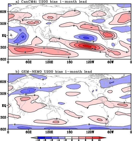
Many previous studies have discussed the importance of the extratropical zonal westerly flow for Rossby wave propagation (e.g., Hoskins and Ambrizzi, 1993Footnote 34). The systematic error of U200 is illustrated in Figure 4. The two models have quite different distributions of U200 bias in the extratropical regions. CanCM4i tends to have overestimated westerlies in the Northern Hemisphere middle latitudes, whereas GEM-NEMO has easterly zonal wind systematic errors.
6. Skill Evaluation of CanSIPSv2 comparing to CanSIPS
The performance of CanSIPSv2 is evaluated in comparison with CanSIPS for the hindcast period 1981-2010. The verification data used are the ERA-interim reanalysis for air temperatures and geopotential height, and the GPCP V2.3 dataset for precipitation.
The skill measures considered are for deterministic forecasts, determined from the ensemble mean of the predicted anomalies. In addition to the global maps for winter and summer forecasts, we consider area averages (over the globe, global land, North America and Canada for temperature and precipitation, over the globe, the Northern Hemisphere extratropics, tropics and Southern Hemisphere extratropics for 500-hPa geopotential height) of anomaly correlation, i.e. the correlation coefficient between predicted and observed anomalies. In addition, in assessing the ensemble forecast skill over Canada, we also discuss the continuous ranked probability skill score (CRPSS; e.g., Bradley and Schwartz 2011Footnote 35) which measures differences between the forecast and observed distributions. A comparison of the skills of the two systems follows.
6.1 Surface air temperature
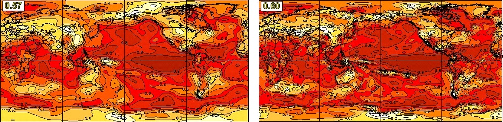
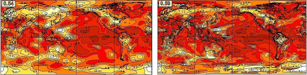
Figure 5 shows the global geographical distribution of anomaly correlation skill for predictions of seasonal mean surface air temperature from the CanSIPS hindcasts (left) and the new CanSIPSv2 hindcasts (right), for the DJF season with zero-month lead. As is usually the case the highest skill for both systems is in the tropics and especially the tropical Pacific, where SST anomalies are most persistent and ENSO imparts relatively high predictability. Skills are also appreciable in many locations over land, including most of North America where much of the seasonal predictability particularly in winter and early spring is attributable to the teleconnected influence of ENSO. In general, the skill distributions of the two systems are comparable. The global average skill of CanSIPSv2 is higher than CanSIPS. Similar conclusion can be obtained for the JJA season (Figure 6), as well as other seasons (not shown).
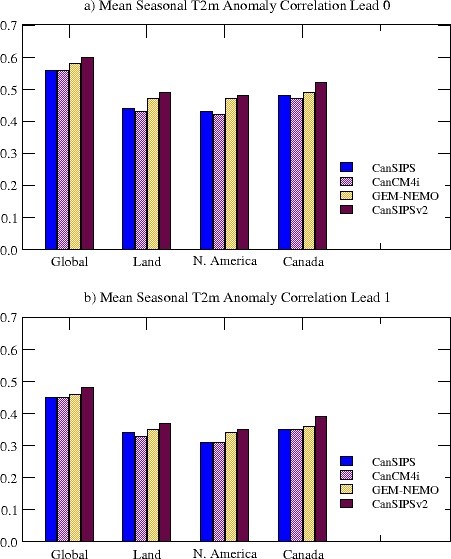
Shown in Figure 7 are T2m anomaly correlation skills for different regions and for lead times of zero month (top) and one month (bottom) averaged over all the 12 initialization months. It is evident that GEM-NEMO alone has a performance comparable to or better than that of CanSIPS. By combining GEM-NEMO with CanCM4i, CanSIPSv2 skill is significantly improved over that of the CanSIPS hindcasts over all the regions.
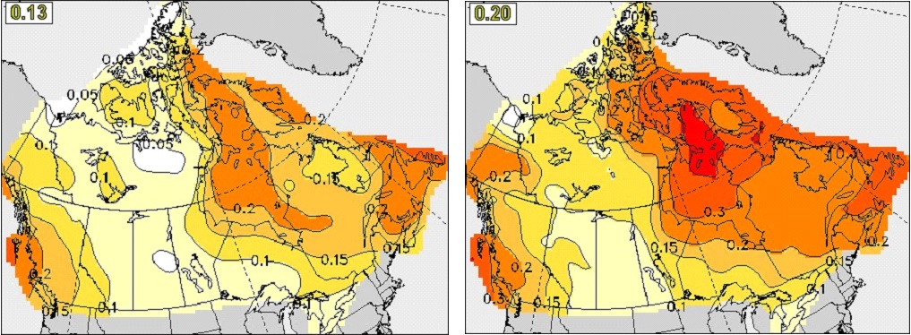
To measure the quality of probability forecasts of the ensemble system, we present in Figure 8 the continuous ranked probability skill score (CRPSS) for DJF seasonal mean T2m forecast at zero month lead in Canada. In both CanSIPS and CanSIPSv2, high skill scores are observed in a large part of northeast Canada and the west coastal regions. Relatively low skill is seen in the Prairies. The CRPSS skill distribution is consistent with the anomaly correlation of the ensemble mean forecast as shown in Figure 5. Comparing the two systems, it is clear that CanSIPSv2 performs better than the previous CanSIPS, especially in eastern Canada. Similar feature of the CRPSS skill scores can be seen for JJA (Figure 9). It is also observed that the skill is improved in CanSIPSv2 comparing to CanSIPS.
6.2 Precipitation
The global distribution of anomaly correlation skill for seasonal mean precipitation forecast in DJF with zero-month lead is shown in Figure 10 for CanSIPS (left) and CanSIPSv2 (right) hindcasts. Again, high skill is mainly observed in the tropical regions, reflecting the contribution of ENSO. Some skill of precipitation is seen in the western and eastern coastal regions of North America. The global average skill of CanSIPSv2 is higher than CanSIPS, although the distributions of the two systems are very similar. For the JJA forecast, the precipitation skill has a similar distribution as DJF but with a weaker magnitude (Figure 11). In this season, both systems produce skillful seasonal precipitation forecasts over western North America. Again, the global average skill of precipitation in CanSIPSv2 is higher than that of CanSIPS.
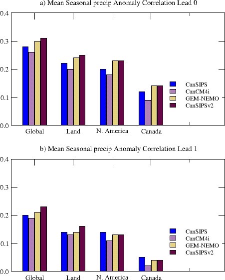
The anomaly correlation skills of precipitation averaged over all 12 initialization months for different regions are illustrated in Figure 12 for lead times of zero month (top) and one month (bottom). In general, the precipitation skill is low, especially for lead-time of one month. It is seen that CanSIPSv2 outperforms CanSIPS in precipitation forecast in all regions for the 0-month lead seasonal forecast. For the one-month lead, we see improvement of precipitation skill over the globe and land but some degradation over North America and Canada, although the skill is very low.
The CRPSS skills for DJF and JJA seasonal mean precipitation forecasts at zero month lead in Canada are shown in Figure 13 and Figure 14, respectively. Although the precipitation forecast skill is low, appreciable improvement in CanSIPSv2 can be identified for DJF. The two systems have comparable CRPSS skill in JJA.
6.3 500-hPa geopotential height
In this section, we evaluate the seasonal forecast skill of 500-hPa geopotential height (Z500). Spatial distributions of the forecast skill for zero lead for the winter season (DJF) and summer season (JJA) are presented.
The anomaly correlation skills for DJF seasonal mean Z500 at zero month lead, i.e., initialized on December 1, are compared between CanSIPS and CanSIPSv2 in Figure 15. Similar to T2m and precipitation, significant skill of Z500 is found in the tropics. In the Northern Hemisphere extratropics, the correlation skill is high over the North Pacific and most part of Canada, resulting from variability of the PNA associated with ENSO (e.g., Wallace and Gutzler 1981Footnote 36). Relatively high correlation skills are also observed over Greenland and the middle latitude North Atlantic, which appears related to the NAO. In general, the two systems have a similar skill distribution. However, the skills over the North Pacific and Greenland region as well as the global average are higher in CanSIPSv2 than in CanSIPS.
For the season of JJA, as can be seen in Figure 16, the forecast skill of seasonal mean Z500 is also high in the tropics. In the Northern Hemisphere extratropics, besides the Greenland and polar regions, four centres of high skill are found in a wave pattern along the middle latitudes, that are eastern Europe, China, the North Pacific and western North America. The last is likely responsible for the high temperature and precipitation skills in western North America as seen in Figure 6 and Figure 11. CanSIPSv2 has a higher global average of skill value than CanSIPS, although the two systems have a very similar skill distribution.
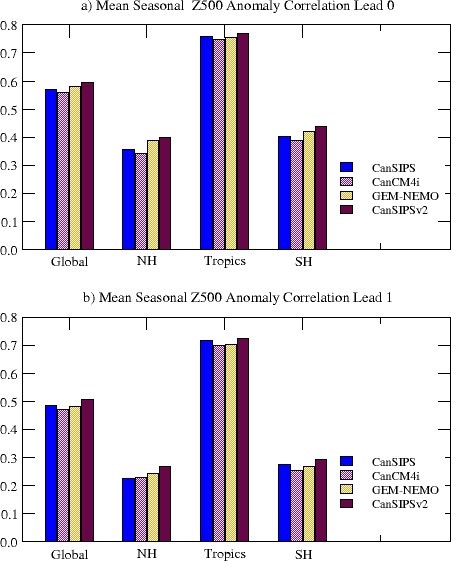
The anomaly correlation skill averaged over all 12 initialization months for different regions, i.e., the globe, the Northern Hemisphere extratropics (30N-90N), the tropics (30S-30N) and the Southern Hemisphere extratropics (30S-90S), are presented in Figure 17 for lead times of zero month (top) and one month (bottom). Again, the CanSIPSv2 system outperforms CanSIPS in all the regions at both the lead times.
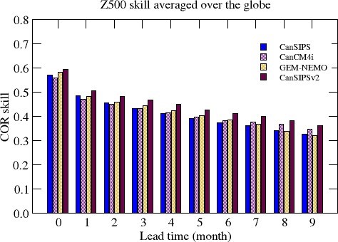
In order to see the skill evolution with the increase of lead time, shown in Figure 18 is the Z500 anomaly correlation skill averaged over the globe as a function of lead time. The skills shown are averages for all 12 initialization months. As can be seen, the improvement of forecast skill of CanSIPSv2 over that of CanSIPS occurs for all lead times.
6.4 SST and ENSO
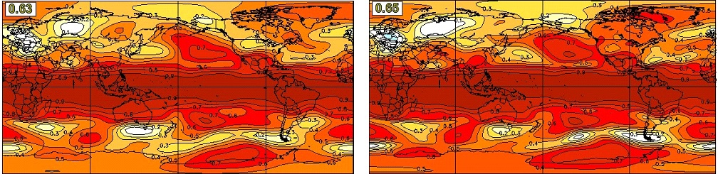
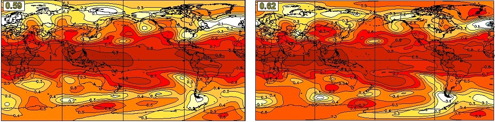
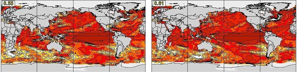
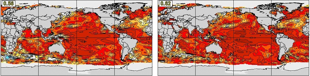
We first show the anomaly correlation skill of DJF seasonal mean SST at one-month lead, i.e., initialized on November 1, in Figure 19. The two systems have a very similar skill distribution. High skill of SST forecast can be found over the global ocean, with the maximum skill in the ENSO region of the equatorial eastern Pacific. The global average skill of CanSIPSv2 (0.61) is higher than that of CanSIPS (0.55). The skill for the one-month lead SST forecast of JJA has a similar distribution as in DJF, but weaker and less concentrated in the ENSO region (Figure 20).
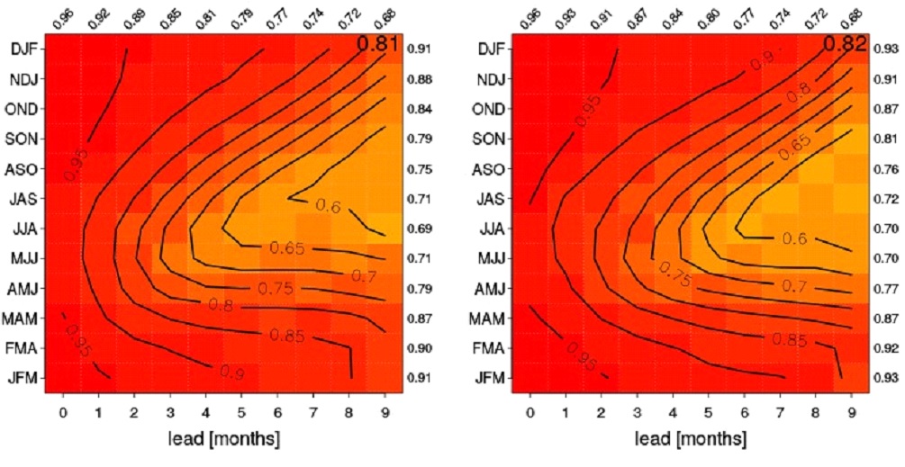
To demonstrate the forecast skill of ENSO, the Nino3.4 index is used which is defined as the SST anomaly averaged in the area of 5°N-5°S, 170°W-120°W. Figure 21 provides a summary of the correlation skill of the seasonal mean Nino3.4 index as a function of target season (vertical axis) and lead time in month (horizontal axis). The skill scores averaged among all the target seasons as a function of lead are printed along the top of the figure, while those averaged among all the lead times as a function of the target season are shown along the right-hand side. The grand average for all the target seasons and lead times is printed at the top-right corner inside the figure. In general, the two systems have comparable ENSO forecast skill. CanSIPSv2 has a slightly better overall skill. For the winter target seasons, CanSIPSv2 shows a better performance. For example, for the DJF and JFM forecasts, the skill of 0.90 for CanSIPSv2 reaches seven-month lead, which is about two months longer than CanSIPS.
6.5 The PNA and NAO
The Pacific-North American pattern and the North Atlantic Oscillation (NAO) are two leading modes of interannual variability of seasonal mean circulation in the Northern Hemisphere extratropics (e.g., Wallace and Gutzler 1981Footnote 36), that greatly influence the weather and climate. Here we analyze the forecast skill of these two patterns.
The PNA and NAO are defined as the first and second rotated empirical orthogonal function (REOF) modes of the monthly mean 500-hPa geopotential height over the Northern Hemisphere using the NCEP/NCAR reanalyses, following Barnston and Livezey (1987)Footnote 37. Monthly mean anomalies for all 12 calendar months are used. Since the PNA and NAO variability has the largest variance in the cold season, the patterns are thus dominated by characteristics in winter. The PNA and NAO indices are calculated as the projections of the seasonal mean 500 hPa geopotential height anomalies onto the respective REOF patterns. In the following discussion, comparisons of PNA and NAO skills are made between CanSIPS and CanSIPSv2. The verification indices are obtained by projecting the corresponding ERA-interim seasonal mean Z500 anomaly onto the PNA and NAO patterns.
The correlation skills of the PNA index as a function of target season are presented in Figure 22 for lead times of zero month (top) and one month (bottom). The PNA skill changes with target season, with high skill in winter, spring to early summer. In late summer and autumn when the PNA is not well defined, the skill is low. In general, the PNA skill of CanSIPSv2 is similar to that of CanSIPS. The wintertime PNA skill is improved in CanSIPSv2 comparing to CanSIPS at the 0-month lead time (Figure 22a). At the one-month lead, however, there is some degradation of wintertime PNA skill, especially for DJF and JFM (Figure 22b).
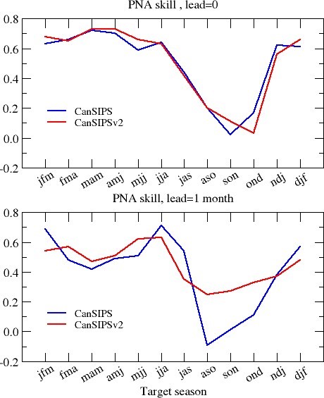
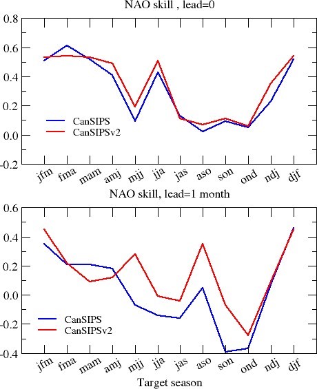
The forecast skill of the NAO index is shown in Figure 23. Relatively high NAO skill is also observed for the winter and spring target seasons. For the forecasts of most target seasons, the CanSIPSv2 system outperforms CanSIPS, especially for the forecasts of one-month lead.
6.6 Sea Ice
CanSIPS was one of the first seasonal prediction systems to have an interactive sea ice model component that in principle enables seasonal predictions of sea ice. In practice CanSIPS Arctic sea ice prediction skill, though appreciable, is attributable mainly to the long-term trend which however tends to be underrepresented in the reforecasts (Sigmond et al., 2013Footnote 20). This suggests considerable room for improvement, and in fact deficiencies in CanSIPS initialization of sea ice have been identified that likely degrade skill. These include unrealistic Arctic sea ice extent trends in the data product used to initialize sea ice concentration in the reforecasts, as well as the use of a seasonally varying model-based climatology having no long-term thinning trend to initialize sea ice thickness.
A further deficiency of sea ice initialization in the CanSIPS reforecasts is that the sea ice concentration (SIC) product that was used is biased low compared to the GDPS analysis, especially during the summer melt season. This contributed to a notable high bias in real time CanSIPS forecasts of Arctic sea ice extent, which were not useful largely for that reason.
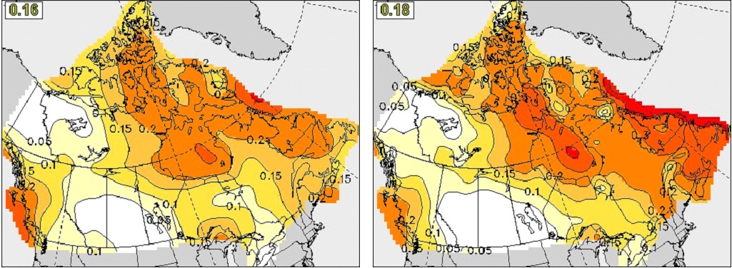
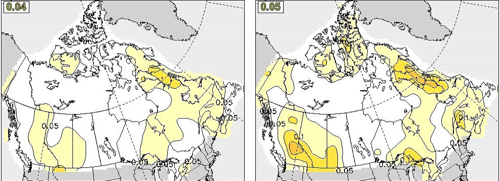
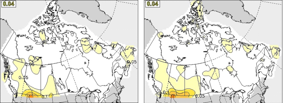
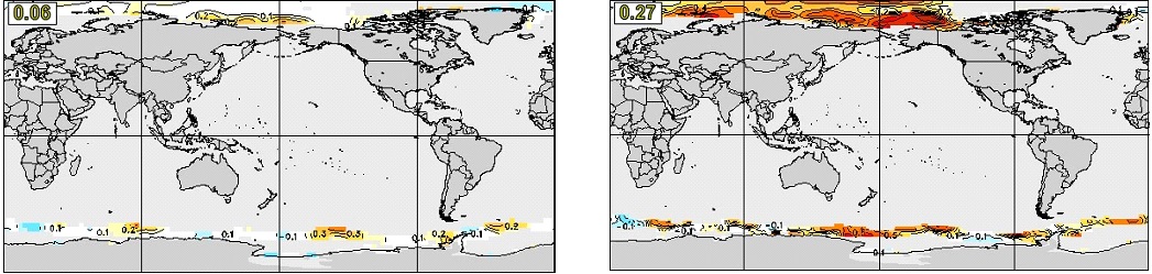
The modifications to the initialization of sea ice in the CanCM4i forecasts and reforecasts described in sections 3.1 and 4.1 are intended to address the above issues and to provide higher forecast skill for sea ice in CanCM4i compared to CanCM4, and to reduce the large biases and resulting errors in real time forecasts. As an example, Figure 24 compares anomaly correlation reforecast skills for prediction of September SIC at four-month lead (initialized at the beginning of May) in CanCM4 and CanCM4i.
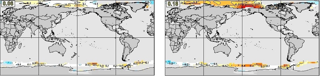
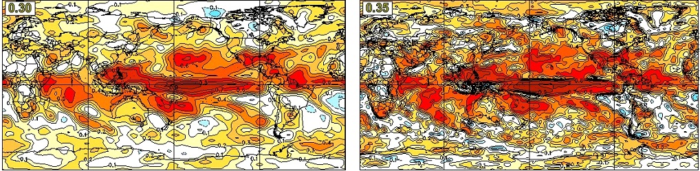
Further improvement in sea ice skill in CanSIPSv2 is provided by GEM-NEMO, which is even more skillful than CanCM4i (e.g. global mean anomaly correlation over ice-covered regions for September SIC at four-month lead near 0.30). This overall improvement is illustrated in Figure 25, which compares anomaly correlation reforecast skills for prediction of September SIC at four-month lead in CanSIPS and CanSIPSv2.
7. Qualitative evaluation of the parallel run
The parallel run of May and June 2019 produced consistent seasonal forecasts with the operational CanSIPS.
8. Details of implementation
An important aspect of any operational seasonal prediction system is that the same model versions and initialization methods are used for producing the forecasts and reforecasts, and both CanSIPSv2 models fulfill this requirement. However, because the MSC analyses employed for initializing the forecasts in real time are not available for the reforecast period, there are inevitably some differences between the data products used for initializing the forecasts and reforecasts, as described in sections 3 and 4. In general, the choice of data products for initializing the reforecasts is guided by considerations of compatibility with the corresponding analyses used in real time. For example, the ORAP5 ocean reanalysis used by both CanSIPSv2 models is formulated using the same modelling system (NEMO) and basic grid (ORCA025) as the GIOPS ocean analysis used for initialization in real time. Also, the Had2CIS sea ice concentration product was developed and chosen for initialization of the reforecasts for both models because it exhibits lower biases relative to the GPDS analysis employed in real time than other products such as ORAP5, which is substantially biased toward lower concentrations than the GPDS product especially in the summer melt season.
An additional aspect of operational CanSIPSv2 that differs from the reforecasts is that, whereas reforecasts are initialized once per month at 00Z on the first day of each month, operational forecasts are initialized and run every day according to the following schedule, with initialization at 00Z in each case:
- 15th day of month: forecast through the remainder of the current month plus six additional months (i.e. six-month forecast with 0.5 month lead), which serves as a mid-month “preview” forecast
- 4th to last day of month: 12-month forecast with 4-day lead, which serves as a backup in the event of an issue with the official forecast
- last day of month: 12-month forecast with 1-day lead, which serves as the official forecast
- every other day: forecast through the remainder of the current month plus one additional month, to track system functioning
Note in particular the 1-day lead time for the official forecasts (as compared to 0-day lead for the reforecasts), which ensures their timely delivery by the start of each month but is unlikely to have any measurable impact on seasonal forecast skill.
Probabilistic offical forecast products are provided at
- https://weather.gc.ca/saisons/index_e.html
- http://climate-scenarios.canada.ca/?page=seasonal-forecasts
As for CanSIPS, these calibrated probabilistic forecasts are post-processed using the methodology described in Kharin et al. (2017)Footnote 38. This improves the reliability of the forecasts, meaning that the forecast probabilities provide a fair measure of the chance of the forecast conditions actually occurring, rather than being over- or under-estimated, as determined from the reforecasts.
9. Summary
The main aspects of the CanSIPSv2 system are summarized as follows
- Like CanSIPS, CanSIPSv2 employs two global atmosphere-ocean-sea ice coupled models to produce multi-model ensemble seasonal predictions. One of the climate models in CanSIPS, CanCM3, was replaced by GEM-NEMO which is an NWP-based coupled model. The remaining climate model in CanSIPS, CanCM4, was upgraded to CanCM4i with improved initialization.
- CanSIPSv2 outperforms CanSIPS in forecasting surface air temperature and 500 hPa geopotential height in all regions for all lead times.
- Although the forecast skill of precipitation is low, CanSIPSv2 has better skill for seasonal mean precipitation forecast at zero-month lead time than CanSIPS.
- The SST and ENSO skill is also improved in CanSIPSv2 comparing to CanSIPS, especially for the Northern Hemisphere winter seasons.
- The NAO skill in CanSIPSv2 is in general higher than CanSIPS. The PNA skill is equivalent in these two systems with slight degradation of skill in winter.
- Significant improvement of sea ice forecast quality is achieved in CanSIPSv2 comparing to the previous system.
10. Acknowledgments
Members of the Seasonal Forum and many colleagues at RPN, CCCma and CMC contributed to the development and implementation of CanSIPSv2. In particular, we would like to thank the following colleagues for their various contributions to this project:
Frédéric Dupont, François Roy, Jean- François Lemieux, Jean-Marc Bélanger, Normand Gagnon, Peter Houtekamer, Ron McTaggart-Cowan, Ayrton Zadra, Paul Vaillancourt, Michel Roch, Stéphane Chamberland, Vivian Lee, Michel Desgagné, Stéphane Bélair, Maria Abrahamowicz, Marco Carrera, Nicola Gasset, Katja Winger.
12. List of Acronyms
| CCCma | Coupled Climate Model, versions 3 |
| CanCM4 | CCCma Coupled Climate Model, versions 4 |
| CanCM4i | CCCma Coupled Climate Model, versions 4, with improved initialization |
| CanSIPS | Canadian Seasonal to Interannual Prediction System |
| CanSIPSv2 | CanSIPS version 2 |
| CCA | Canonical Correctional Analysis |
| CCCma | Canadian Centre for Climate Modeling and Analysis |
| CIS | Canadian Ice Service |
| Cice | Community of Ice CodE |
| CMC | Canadian Meteorological Centre |
| CONCEPTS | The Canadian Operational Network of Coupled Environmental PredicTion Systems |
| CRPSS | Continuous Rank probability Skill Score |
| ECCC | Environment and Climate Change Canada |
| EnKF | Ensemble Kalman Filter |
| ENSO | El Niño/Southern Oscillation |
| GDPS | Global Deterministic Prediction System |
| GEM | Global Environmental Multiscale model |
| GEM-NEMO | GEM and NEMO coupled model |
| GEPS | Global Ensemble Prediction System |
| GIOPS | Global Ice Ocean Prediction System |
| GOSSIP | Globally Organized System for Simulation Information Passing |
| GPCP | Global Precipitation Climatology Project |
| Had2CIS | HadISST2 combined with CIS digitized sea ice charts |
| HadISST2 | Hadley Centre Sea Ice and Sea Surface Temperature Version 2 |
| HFP | Historical Forecast Project |
| NEMO | Nucleus for European Modelling of the Ocean |
| MSC | Meteorological Service of Canada (of Environment Canada) |
| NAO | North Atlantic Oscillation |
| NCAR | National Center for Atmospheric Research |
| NCEP | (United States) National Centers for Environmental Prediction |
| NOAA | National Oceanic and Atmospheric Administration |
| NWP | Numerical Weather Prediction |
| PNA | Pacific/North American pattern |
| OISST | Optimum Interpolation Sea Surface Temperature of NOAA |
| ORAP5 | Ocean Reanalyses Prototype 5 |
| ORAS5 | Ocean Reanalysis System 5 |
| RPN | Recherche en Prévision Numérique |
| REOF | Rotated Empirical Orthogonal Function |
| SIC | Sea Ice Concentration |
| SPS | Surface Prediction System |
| SST | Sea Surface Temperature |
| T2m | 2-meter air temperature |
| Z500 | 500-hPa geopotential height |