
The ensemble of daily predictor variables developed from the CanESM2 CMIP5 experiments
On this page
Introduction
The main goal of this project was to develop the ensemble of daily predictors using output variables from the CanESM2 experiments as prepared for the Coupled Model Intercomparison Project Phase 5 (CMIP5). The ensemble includes the 25 basic predictor variables as well as total precipitation amount at the daily scale (see below). They are defined on the global Gaussian reduced grid associated with spectral truncation T42 that consists of 128x64 grid cells in longitude-latitude direction. For the purposes of model calibration and validation, the 26 predictors having the same characteristics as those based on the CanESM2 output are developed from the NCEP/NCAR reanalysis.
A secondary objective was to design a fast and cost-effective approach to develop the predictors using global time series of data as stored in NetCDF format. A short description of the data sources is available in section 1. The methodology of the development and organization of predictor files is available in section 2.
1. Description of input data
1.1 CanESM2 global climate model
The second generation of Earth System Model CanESM2 (von Salzen et al., 2005Footnote 6; Li and Barker., 2005Footnote 3; Barker et al., 2005Footnote 1) is the fourth generation of the coupled global climate model (i.e. CGCM4) developed by the Canadian Centre for Climate Modelling and Analysis (CCCma) of Environment and Climate Change Canada. CanESM2 represents a part of the Canadian modelling community's contribution to the IPCC Fifth Assessment Report (AR5). Main components of the Earth System Model include: (i) Atmospheric General Circulation Model (AGCM4) having triangular truncation resolution T63 with the hybrid vertical domain expanded in 35 vertical layers; (ii) Ocean GCM4 developed from the NCAR CSM Ocean Model and defined by 256x192 horizontal resolution and 40 vertical layers; (iii) CanSim1 sea-ice model; and (iv) Canadian Land Surface Scheme (CLASS2.7) and CTEM1 for land processes. For more details on CanESM2 and its components, please visit CCCma’s webpage.
For the purposes of the development of the suggested set of predictors, the atmospheric variables (see section 2.1) from the first member run (r1i1p1) have been selected. The past climate conditions over the 1961-2005 period are represented by the historical simulation. As for the projections of future changes in climate based on the period 2006-2100, new scenarios developed for the IPCC AR5 are introduced. The emissions, concentrations, and land-cover change projections are described by the Representative Concentration Pathways scenarios such as RCP2.6, RCP4.5 and RCP8.5 (Moss et al., 2010Footnote 5; Meinshausen et al., 2011Footnote 4).
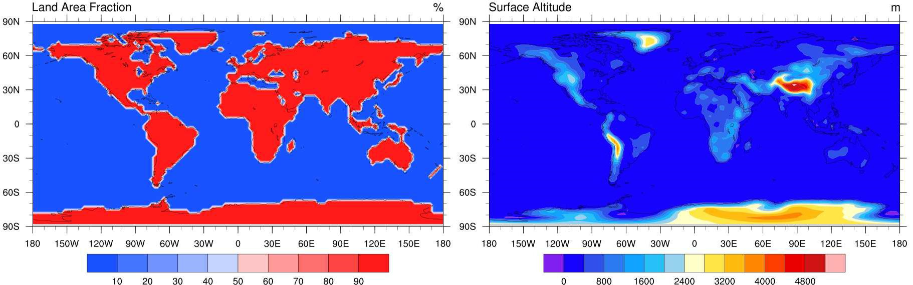
Since CanESM2 is a member of the CMIP5 project, atmospheric variables issued from aforementioned runs are available on the T42 (see Figure 1) instead of T63 grid projection. Spatial interpolation from T63 to T42 grid has been performed and made available online by CCCma. Since daily GCM data are required for the construction of predictors, the upper-level fields were selected as daily mean over four time steps. The near-surface fields have already been defined as daily variables. For access to available atmospheric fields as simulated by CanESM2 AGCM4, please visit CCCma's page on climate model graphics.
1.2 NCEP/NCAR Reanalysis 1
The NCEP/NCAR Reanalysis Project 1 (Kalnay et al., 1996Footnote 2) is a result of collaboration between National Centers for Environmental Prediction (NCEP) and National Center for Atmospheric Research (NCAR). These global atmospheric reanalysis datasets are based on the state-of-art assimilation/forecast system of high-density historical observations (from 1948 to present).
To keep things consistent with the raw atmospheric variables available from CanESM2 outputs, the same variables were selected from NCEP/NCAR. The historical reference time frame ranges from the years 1961 to 2005. The variables defined at pressure levels as well as mean sea level pressure were available on the global regular latitude-longitude grid projection of 2.5 degrees. However, 2m air temperature and total precipitation were available on the finer spatial resolution, global Gaussian T62 grid projection (94 latitudes x 192 longitudes). Corresponding latitudes have been defined in an inverse order, north to south, compared to the CanESM2 output grid.
Visit NCEP/NCAR to access the NCEP/NCAR Reanalysis project 1 results and available variables.
2. Methodology
2.1 Raw and derived variables
Global daily time series of variables described as raw data in Table 1 are provided from both data sources (CanESM2 and NCEP/NCAR) in NetCDF format. Each dataset has undergone first only minimal preprocessing to ensure consistency in structure of the input files during standardization and extraction to grid boxes. An ensemble of codes created for data manipulation and selection of predictors was executed on Linux system in Bourne Advanced Shell (bash) environment. Data interpolation and predictor selection are based on the NCAR Command Language (NCL) version 6.1.2. NCL is an interpreted language developed by NCAR and designed specifically for scientific data analysis and visualization.
For the CanESM2 outputs, preprocessing consists of:
- Separating multi-yearly to yearly files;
- Selecting upper-air variables from desired pressure levels (1000, 850 and 500 hPa);
- Adjusting values in time arrays so that time monotonically increases following Julian days as needed for later selection of gridded data per grid box (section 2.2);
- Converting variables to double precision, and Kelvin to degrees Celsius (for temperature).
The NCEP/NCAR raw variables were also available in NetCDF format. Preprocessing of reanalysis raw data includes spatial interpolation to the global Gaussian grid T42 of CanESM2 after level selection for the upper-air variables. For that purpose, the NCL’s built-in function f2gsh_Wrap was applied. The function is based on spherical harmonics and interpolates a scalar field from a fixed (i.e. regular latitude-longitude grid) to a Gaussian grid. Spatial coverage of NCEP/NCAR data is considered as fixed or regular grid because the distance between two consecutive grid points is the same in the latitude/longitude direction.
Therefore, the second part of predictor development consists of computing the air flow variables from zonal and meridional wind components defined on the T42 Gaussian grid. The calculation is based on the NCL built-in functions as identified in Table 1. Here, divergence and relative vorticity are based on true wind since this variable is available from both data sources.
Table 1: Basic description of predictor variables derived from raw data of CanESM2 and NCEP/NCAR.
| Variable | Unit | Level | Type |
|---|---|---|---|
| Total precipitation | mm | surface | Raw |
| Air temperature | °C | 2m | Raw |
| Mean sea level pressure | Pa | Mean sea level | Raw |
| Specific humidity | kg/kg | Pressure levels | Raw |
| Geopotential height | m | Pressure levels | Raw |
| Zonal wind | m/s | Pressure levels | Raw |
| Meridional wind | m/s | Pressure levels | Raw |
| Wind speed1 | m/s | Pressure levels | - |
| Wind direction1,2 | 0-360° | Pressure levels | wind_direction |
| Divergence1 | Pressure levels | uv2dvG_Wrap | |
| Relative vorticity1 | Pressure levels | uv2vrG_Wrap |
1Derived using NCL function. 2Wind direction (calculated from U and V components) in degrees corresponds to: 0° pointing north, 90° pointing east, 180° pointing south and 270° pointing west.
2.2 Characteristics of grid-box directories
The 26 variables are first standardized against the corresponding historical reference period (for each source of data, i.e. with respect to CanESM2 baseline for CanESM2 predictors and with respect to NCEP/NCAR baseline for NCEP/NCAR predictors) and then organized per grid box into 1-column text files per data source per variable. In this case, standardization of the global daily time series is based on long-term climate mean and its standard deviation over the 1971 to 2000 reference period. Then, except for wind direction, all predictor values (x), for both the historical and future periods, have been normalised (n) with respect to the means (µ) and standard deviations () of the 1971-2000 reference period using the following expression:
The name of the five directories containing each grid box for the baseline and future periods from both NCEP/NCAR and CanESM2 are listed in Table 2. Note that the corresponding RCP scenario for each CanESM2 run is stated before the information of the time window (i.e. rcp26 for RCP2.6 scenario, rcp45 for RCP4.5 scenario, and rcp85 for RCP8.5 scenario).
2.2.1 Structure of predictor files
Long-term time series of standardized daily values (and wind direction) are then extracted into a one column text file per grid cell (box). The 128x64 grid cells cover the global domain according to T42 Gaussian grid. This grid is uniform along the longitude with horizontal resolution of 2.8125° and is nearly uniform along the latitude of roughly 2.8125° (see Table 3). The predictors associated with each grid cell are represented by corresponding folder named BOX_iiiX_jjY, where iii=1,128 is the longitudinal index and jj=1,64 is the latitudinal index. The structure of these folders is described in Table 2. The predictors organized in this way are ready for use as input in the statistical downscaling models such as ASD or SDSM.
Table 2: Structure of a BOX_iiiX_jjY folder: the two auxiliary text files and five sub-folders where each are containing the 26 predictor files issued from selected source of data.
| Two auxiliary files providing details on a given grid cell (see Figure 1) | ||
|---|---|---|
| gauss42_sftlf.txt | Land-area fraction [%] | 0 % if oceanic and Great Lakes grid points; 100% if land and small inland |
| gauss42_orog.txt | Orography [m] | Surface altitude |
| Five sub-folders for data type | Time frame | The 4-characters acronym |
|---|---|---|
| NCEP-NCAR_1961_2005 | 1961 to 2005 | ncep |
| CanESM2_historical_1961_2005 | 1961 to 2005 | cesh |
| CanESM2_rcp26_2006_2100 | 2066 to 2100 | ces2 |
| CanESM2_rcp45_2006_2100 | 2066 to 2100 | ces4 |
| CanESM2_rcp85_2006_2100 | 2066 to 2100 | ces8 |
Each sub-folder contains the 26 files of predictors. A filename consists of 10 characters with extension .dat. The list of filenames is given in Table 4: The P* points to a 4-character prefix as given in Table 2, then predictor name is identified using the 5th to 8th character, and gl stands for global grid.
Table 3: Latitude / longitude cell numbering for the Gaussian 128x64 grid: The latitudes are numerated from south to north and represent grid index associated with Y (64 values). The longitudes are numerated from the Greenwich meridian toward east (associated with 128 X values).
| N° of Y and its corresponding latitude | ||||||||
|---|---|---|---|---|---|---|---|---|
| jj (Y) | 1 | 2 | 3 | 4 | ||||
| Latitude | 87.863°S | 85.096°S | 82.312°S | 79.525°S | ||||
| jj (Y) | 5 | 6 | 7 | 8 | ||||
| Latitude | 76.736°S | 73.947°S | 71.157°S | 68.367°S | ||||
| jj (Y) | 9 | 10 | 11 | 12 | ||||
| Latitude | 65.577°S | 62.787°S | 59.997°S | 57.206°S | ||||
| jj (Y) | 13 | 14 | 15 | 16 | ||||
| Latitude | 54.416°S | 51.625°S | 48.835°S | 46.044°S | ||||
| jj (Y) | 17 | 18 | 19 | 20 | ||||
| Latitude | 43.254°S | 40.463°S | 37.673°S | 34.882°S | ||||
| jj (Y) | 21 | 22 | 23 | 24 | ||||
| Latitude | 32.091°S | 29.301°S | 26.510°S | 23.720°S | ||||
| jj (Y) | 25 | 26 | 27 | 28 | ||||
| Latitude | 20.929°S | 18.138°S | 15.348°S | 12.557°S | ||||
| jj (Y) | 29 | 30 | 31 | 32 | ||||
| Latitude | 9.767°S | 6.976°S | 4.185°S | 1.395°S | ||||
| jj (Y) | 33 | 34 | 35 | 36 | ||||
| Latitude | 1.395°N | 4.185°N | 6.976°N | 9.767°N | ||||
| jj (Y) | 37 | 38 | 39 | 40 | ||||
| Latitude | 12.557°N | 15.348°N | 18.138°N | 20.929°N | ||||
| jj (Y) | 41 | 42 | 43 | 44 | ||||
| Latitude | 23.720°N | 26.510°N | 29.301°N | 32.091°N | ||||
| jj (Y) | 45 | 46 | 47 | 48 | ||||
| Latitude | 34.882°N | 37.673°N | 40.463°N | 43.254°N | ||||
| jj (Y) | 49 | 50 | 51 | 52 | ||||
| Latitude | 46.044°N | 48.835°N | 51.625°N | 54.416°N | ||||
| jj (Y) | 53 | 54 | 55 | 56 | ||||
| Latitude | 57.206°N | 59.997°N | 62.787°N | 65.577°N | ||||
| jj (Y) | 57 | 58 | 59 | 60 | ||||
| Latitude | 68.367°N | 71.157°N | 73.947°N | 76.736°N | ||||
| jj (Y) | 61 | 62 | 63 | 64 | ||||
| Latitude | 79.525°N | 82.312°N | 85.096°N | 87.863°N | ||||
| N° of X(iii) | Longitude(°East) |
|---|---|
| 1 | 0 |
| 2 | 2.8125 |
| 3 | 5.625 |
| 4 | 8.4375 |
| 5 | 11.25 |
| 6 | 14.0625 |
| 7 | 16.875 |
| 8 | 19.6875 |
| 9 | 22.5 |
| 10 | 25.3125 |
| 11 | 28.125 |
| 12 | 30.9375 |
| 13 | 33.75 |
| 14 | 36.5625 |
| 15 | 39.375 |
| 16 | 42.1875 |
| 17 | 45 |
| 18 | 47.8125 |
| 19 | 50.625 |
| 20 | 53.4375 |
| 21 | 56.25 |
| 22 | 59.0625 |
| 23 | 61.875 |
| 24 | 64.6875 |
| 25 | 67.5 |
| 26 | 70.3125 |
| 27 | 73.125 |
| 28 | 75.9375 |
| 29 | 78.75 |
| 30 | 81.5625 |
| 31 | 84.375 |
| 32 | 87.1875 |
| 33 | 90 |
| 34 | 92.8125 |
| 35 | 95.625 |
| 36 | 98.4375 |
| 37 | 101.25 |
| 38 | 104.0625 |
| 39 | 106.875 |
| 40 | 109.6875 |
| 41 | 112.5 |
| 42 | 115.3125 |
| 43 | 118.125 |
| 44 | 120.9375 |
| 45 | 123.75 |
| 46 | 126.5625 |
| 47 | 129.375 |
| 48 | 132.1875 |
| 49 | 135 |
| 50 | 137.8125 |
| 51 | 140.625 |
| 52 | 143.4375 |
| 53 | 146.25 |
| 54 | 149.0625 |
| 55 | 151.875 |
| 56 | 154.6875 |
| 57 | 157.5 |
| 58 | 160.3125 |
| 59 | 163.125 |
| 60 | 165.9375 |
| 61 | 168.75 |
| 62 | 171.5625 |
| 63 | 174.375 |
| 64 | 177.1875 |
| 65 | 180 |
| 66 | 182.8125 |
| 67 | 185.625 |
| 68 | 188.4375 |
| 69 | 191.25 |
| 70 | 194.0625 |
| 71 | 196.875 |
| 72 | 199.6875 |
| 73 | 202.5 |
| 74 | 205.3125 |
| 75 | 208.125 |
| 76 | 210.9375 |
| 77 | 213.75 |
| 78 | 216.5625 |
| 79 | 219.375 |
| 80 | 222.1875 |
| 81 | 225 |
| 82 | 227.8125 |
| 83 | 230.625 |
| 84 | 233.4375 |
| 85 | 236.25 |
| 86 | 239.0625 |
| 87 | 241.875 |
| 88 | 244.6875 |
| 89 | 247.5 |
| 90 | 250.3125 |
| 91 | 253.125 |
| 92 | 255.9375 |
| 93 | 258.75 |
| 94 | 261.5625 |
| 95 | 264.375 |
| 96 | 267.1875 |
| 97 | 270 |
| 98 | 272.8125 |
| 99 | 275.625 |
| 100 | 278.4375 |
| 101 | 281.25 |
| 102 | 284.0625 |
| 103 | 286.875 |
| 104 | 289.6875 |
| 105 | 292.5 |
| 106 | 295.3125 |
| 107 | 298.125 |
| 108 | 300.9375 |
| 109 | 303.75 |
| 110 | 306.5625 |
| 111 | 309.375 |
| 112 | 312.1875 |
| 113 | 315 |
| 114 | 317.8125 |
| 115 | 320.625 |
| 116 | 323.4375 |
| 117 | 326.25 |
| 118 | 329.0625 |
| 119 | 331.875 |
| 120 | 334.6875 |
| 121 | 337.5 |
| 122 | 340.3125 |
| 123 | 343.125 |
| 124 | 345.9375 |
| 125 | 348.75 |
| 126 | 351.5625 |
| 127 | 354.375 |
| 128 | 357.1875 |
Table 4: List of the 26 predictor filenames and their corresponding variable names. The prefix P* is defined in Table 2.
| No | File name | Predictor names or variables |
|---|---|---|
| 1 | P*mslpgl.dat | Mean sea level pressure |
| 2 | P*p1_fgl.dat | 1000 hPa Wind speed |
| 3 | P*p1_ugl.dat | 1000 hPa Zonal wind component |
| 4 | P*p1_vgl.dat | 1000 hPa Meridional wind component |
| 5 | P*p1_zgl.dat | 1000 hPa Relative vorticity of true wind |
| 6 | P*p1thgl.dat | 1000 hPa Wind direction |
| 7 | P*p1zhgl.dat | 1000 hPa Divergence of true wind |
| 8 | P*p500gl.dat | 500 hPa Geopotential |
| 9 | P*p5_fgl.dat | 500 hPa Wind speed |
| 10 | P*p5_ugl.dat | 500 hPa Zonal wind component |
| 11 | P*p5_vgl.dat | 500 hPa Meridional wind component |
| 12 | P*p5_zgl.dat | 500 hPa Relative vorticity of true wind |
| 13 | P*p5thgl.dat | 500 hPa Wind direction |
| 14 | P*p5zhgl.dat | 500 hPa Divergence of true wind |
| 15 | P*p850gl.dat | 850 hPa Geopotential |
| 16 | P*p8_fgl.dat | 850 hPa Wind speed |
| 17 | P*p8_ugl.dat | 850 hPa Zonal wind component |
| 18 | P*p8_vgl.dat | 850 hPa Meridional wind component |
| 19 | P*p8_zgl.dat | 850 hPa Relative vorticity of true wind |
| 20 | P*p8thgl.dat | 850 hPa Wind direction |
| 21 | P*p8zhgl.dat | 850 hPa Divergence of true wind |
| 22 | P*prcpgl.dat | Total precipitation |
| 23 | P*s500gl.dat | 500 hPa Specific humidity |
| 24 | P*s850gl.dat | 850 hPa Specific humidity |
| 25 | P*shumgl.dat | 1000 hPa Specific humidity |
| 26 | P*tempgl.dat | Air temperature at 2 m |
Data origin
- CanESM2 output data provided by the CCCma, ECCC: http://climate-modelling.canada.ca/climatemodeldata/data.shtml
- NCEP Reanalysis data provided by the NOAA/OAR/ESRL PSD, Boulder, Colorado, USA