
Climate-Resilient Buildings and Core Public Infrastructure: an assessment of the impact of climate change on climatic design data in Canada
User information
The report provides an assessment of how climatic design data relevant to users of the National Building Code of Canada (NBCC 2015, Table C-2) and the Canadian Highway Bridge Design Code (CHBDC/CSA S6 2014, Annex A3.1) might change as the climate continues to warm.
Design decisions should always be made following the appropriate codes and standards. It is important to note that it remains the responsibility of the users of these climatic data to determine whether it is suitable for their particular purpose.
Recommended citation: Cannon, A.J., Jeong, D.I., Zhang, X., and Zwiers, F.W., (2020): Climate-Resilient Buildings and Core Public Infrastructure: An Assessment of the Impact of Climate Change on Climatic Design Data in Canada; Government of Canada, Ottawa, ON. 106 p.
On this page
- Introduction
- Background and methods
- Temperature
- Precipitation and moisture
- Wind pressures
- Snow and ice
- Summary and conclusions
- References
-
Appendices
-
Appendix 1
- Appendix 1.1: Timing of global warming
-
Appendix 1.2: Projected changes
- National Building Code of Canada (NBCC)
- Canadian Highway Bridge Design Code (CHBDC)
- Appendix 2: Links to published papers
-
Appendix 1
- List of acronyms
- Footnotes
1. Introduction
1.1 Context
Climate change is an enormous long-term challenge that faces all countries. It presents a real threat to Canada’s Buildings and Core Public Infrastructure (B&CPI), which includes buildings, bridges, roads, transit systems, potable water, storm water and sanitary sewage systems. The threat includes the possibility of increases in the frequency and intensity of certain extreme weather events, such as rainstorms and flooding, and other hazards that could result in infrastructure damage and failure. There are limitations in the current approaches used for the design and rehabilitation of Canada’s B&CPI as they are based on historical climatic loads. These loads may not be representative of those that could be experienced in a future, warmer, climate. Failure to account for changes in climatic loads could therefore lead to more frequent early failure of elements of Canada’s B&CPI. The consequences of infrastructure failures can be quite significant, including fatalities, injuries, and illnesses, disruption or loss of service, increased costs to infrastructure owners, unforeseen costs to infrastructure users, and considerable negative socioeconomic impacts to the municipal, provincial/territorial and federal governments.
The risk of failure of any of the systems mentioned above depends on both the loads on the system and its resistance to those loads. Both depend on the climate through factors termed climatic loads, including those due to temperature, rain, snow, wind, ice, etc. B&CPI systems are typically designed for long service lives that could vary between 50 and 100 years, and thus they will be exposed to changing climatic loads over their service lives. It is therefore necessary to assess projections of how climate change may affect future climatic loads.
With this in mind, this chapter begins with a brief summary of the current state of understanding about observed and projected changes in temperature, precipitation, and the cryosphere in Canada. This information is extracted from a comprehensive assessment performed by ECCC as part of Canada’s Changing Climate Report (CCCR):
Bush, E. and Lemmen, D.S. (Eds.) (2019): Canada’s Changing Climate Report. Government of Canada, Ottawa, Ontario. 444 p. https://changingclimate.ca/CCCR2019/
Key findings from the CCCR provide the background for the remainder of this report, which provides an assessment of how the climatic design data relevant for developing Canada’s B&CPI may change as the climate continues to warm.
Temperature
It is virtually certainFootnote 1i that Canada’s climate has warmed and that it will warm further in the future. Both the observed and projected increases in mean temperature in Canada are about twice the corresponding increases in the global mean temperature, regardless of emission scenario.
Annual and seasonal mean temperatures across Canada have increased, with the greatest warming occurring in winter. Between 1948 and 2016, the best estimate of mean annual temperature increase is 1.7°C for Canada as a whole and 2.3°C for northern Canada.
While both human activities and natural variations in the climate have contributed to the observed warming in Canada, the human factor is dominant. It is likely that more than half of the observed warming in Canada is due to the influence of human activities.
Annual and seasonal mean temperatures are projected to increase everywhere, with much larger changes in northern Canada in winter. Averaged over the country, warming projected in a low emission scenario is about 2°C higher than the 1986–2005 reference period used in the CCCR, remaining relatively steady after 2050, whereas in a high emission scenario, temperature increases will continue, reaching more than 6°C by the late 21st century.
Future warming will be accompanied by a longer growing season, fewer heating degree days, and more cooling degree days.
Changes in extreme temperatures, both in observations and future projections, are consistent with warming. Extreme warm temperatures have become hotter, while extreme cold temperatures have become less cold. Such changes are projected to continue in the future, with the magnitude of change proportional to the magnitude of mean temperature change.
Precipitation
There is medium confidence that annual mean precipitation has increased, on average, in Canada, with larger percentage increases in northern Canada. Such increases are consistent with model simulations of anthropogenic climate change.
Annual and winter precipitation amounts are projected to increase everywhere in Canada over the 21st century, with larger percentage changes in northern Canada. Summer precipitation is projected to decrease over southern Canada under a high emission scenario toward the end of the 21st century, but only small changes are projected under a low emission scenario.
For Canada as a whole, observational evidence of changes in daily and short- duration extreme precipitation is lacking. However, in the future, daily extreme precipitation is projected to increase (high confidence).
Snow and Ice
The portion of the year with snow cover has decreased across most of Canada by 5% to 10% per decade since 1981, due to later snow onset and earlier spring melt (very high confidence). Seasonal snow accumulation also decreased by 5% to 10% per decade, with the exception of southern Saskatchewan, and parts of Alberta and British Columbia (increases of 2% to 5% per decade) (medium confidence).
It is very likely that snow cover duration will decline to mid-century over Canada due to increases in surface air temperature under all emissions scenarios. Differences in spring snow cover projections between emissions scenarios emerge by end of century, with stabilized snow loss for a moderate emissions scenario but continued snow loss under a high emissions scenario. A reduction of 5% to 10% per decade in seasonal snow accumulation (through 2050) is projected over much of southern Canada; only small changes in snow accumulation are projected over northern regions of Canada because increases in winter precipitation are expected to offset a shorter snow accumulation period (medium confidence).
Observations show increases in permafrost temperature (about 0.1°C per decade in the central Mackenzie Valley; 0.3 to 0.5°C per decade in the high Arctic, over the past 3-4 decades) and active layer thickness (approximately 10% since 2000 in Mackenzie Valley) (high confidence), and widespread formation of themokarst landforms across northern Canada (medium confidence).
Projected increases in mean air temperature over land underlain with permafrost in all emissions scenarios are virtually certain to result in continued permafrost warming and thawing over large areas by mid-century, with impacts on northern infrastructure and the role of northern terrestrial ecosystems in the carbon cycle.
1.2 Approach to the assessment of projected climatic design value changes
The focus of this report is to assess, at a regional-to-national scale, projected changes in the climatic design data that are defined in NBCC 2015 (NRC, 2015)Reference 1 and CHBDC CSA S6 (CSA, 2014)Reference 2 – these are the data that are widely used by engineers to calculate the climatic loads affecting Canada’s B&CPI.
Canada’s Changing Climate Report (CCCR; Bush and Lemmen, 2019)Reference 3 provides a detailed scientific assessment of historical trends and the projected future state of Canada’s surface temperature, precipitation, and cryosphere. In many cases, the specific quantities assessed in the CCCR are the same as the climatic design variables required for infrastructure codes and standards, for example heating degree days, annual total precipitation, and one-day rain. More generally, the Intergovernmental Panel on Climate Change (IPCC) Working Group I regularly conducts comprehensive scientific assessments of the current understanding of the physical science basis of global and regional climate change, most recently summarized in the 5th Assessment Report of IPCC Working Group I (IPCC, 2013)Reference 4Footnote 2ii.
The approach taken in this report is founded, most importantly, on an assessment of the current understanding of climate change from these national and international assessments, as well as in other relevant literature. This assessment is supplemented by ongoing research efforts within Environment and Climate Change Canada’s Climate Research Division (ECCC’s CRD) and elsewhere, and by targeted research conducted specifically for this project.
As noted in the key findings from CCCR, scientific confidence in climate change projections varies depending on the climate variable and, in some cases, region. For example, confidence in temperature change is higher than confidence in precipitation change, in large part because temperature change is a direct consequence of the radiative imbalance associated with changing GHG and aerosol emissions. On the other hand, precipitation change is affected by a number of complex processes including increases in the water holding capacity of a warming atmosphere, changes in global atmospheric circulation, interactions with topography, changes in evaporation, etc. Further, confidence about changes in compound events, involving multiple variables, e.g., snow loads, driving rain wind pressures, etc., is lower than for the individual constituent variables. Given the varying levels of advancement of scientific understanding for the different climatic design elements relevant to B&CPI design, we adopt a multi-tiered approach to the projection of design value changes.
In pursuing the goals of this report, climatic design variables have been grouped into three tiers according to our confidence in their future projections for large regions of Canada, based on judgements about the body of evidence that is available, including published literature both in Canada and abroad, and supplemented by evidence from targeted research based on Canadian climate model simulations:
Tier 1 variables are those for which there is generally high or very high confidence in the future projections for a given level of global warming. This level of confidence is afforded by in-depth understanding of the processes involved, as well as an abundant and a strong body of evidence (including evidence for other parts of the world) that deals with the causes of observed changes. This implies relatively high confidence in projected change factors for these variables, which suggests that specific values of these change factors could be considered when designing new infrastructure if justified from an engineering perspective and if suitable approaches exist to consider remaining uncertainties, including uncertainty in the amount of warming that might occur by the end of the service life of the structure that is being designed.
Tier 2 variables are those for which there is generally medium confidence in the future projections for a given level of global warming. In most instances, an assessment of medium confidence means there is some understanding of the processes that lead to future change. This might be supplemented by a body of evidence linking the causes of observed changes at large scales, but generally, such evidence would be much less extensive, with available studies showing a lower degree of consistency, than for Tier 1 variables. In contrast to situations when climate scientists have high or very high confidence, climate scientists are generally not able to estimate the likelihood of a projected change when they determine that they have medium confidence in future projections. Change factors for these variables are therefore more suitable for cost/benefit analyses or for a risk analysis, as well as for the exploration of uncertainty associated with design.
Tier 3 variables are those for which there is low or very low confidence in the future projections for a given level of global warming. Low or very low confidence is given to projections for variables that have not been widely studied in the published literature or for which the processes involved are poorly understood. In some instances, very low confidence is given to projections for variables that are diagnosed indirectly, for example, using empirical relationships because process understanding is limited. While change factors are projected, they are likely best suited to exploring the potential impacts of climate change on structural reliability in different warming and load combination scenarios.
The specific NBCC (NRC, 2015)Reference 1 and CHBDC (CSA S6, 2014)Reference 2 climatic design variables covered here, and their grouping into tiers, include:
-
heating degree days (NBCC, Tier 1)
-
hourly design temperatures (January 2.5% dry bulb, January 1% dry bulb, July 2.5% dry bulb, and July 2.5% wet bulb) (NBCC, Tier 1)
-
maximum and minimum mean daily air temperatures (CHBDC, Tier 1)
Chapter 4 - Precipitation and moisture
-
annual total precipitation and annual total rainfall (NBCC, Tier 2)
-
annual maximum 1-day rain (50-yr return period) (NBCC, Tier 2)
-
annual maximum 15-min rainfall (10-yr return period) (NBCC, Tier 2)
-
annual mean relative humidity (NBCC and CHBDC, Tier 3)
-
annual maximum hourly wind pressures (10, 25, 50, and 100-yr return periods) (NBCC, and CHBDC, Tier 3)
-
annual maximum driving rain wind pressures (5-yr return period) (NBCC>, Tier 3)
-
annual maximum snow load (50-yr return period) (NBCC, Tier 3)
-
annual maximum ice accretion on exposed surfaces (CHBDC, 20-yr return period) (Tier 3)
-
permafrost region (CHBDC, Tier 3)
Interpretation of the projected design value changes should always take the level of scientific confidence in the projections into account. It should be noted that confidence becomes lower as projections become more specific. For example, lower confidence is associated with local/site specific projections than for corresponding regional, national, or global projections. This is because local scale projections are much more likely to be affected by incomplete process knowledge, and errors in the approximation of the effects of processes that climate models cannot represent explicitly. Also, higher confidence can often be associated with the direction of a projected change than with its magnitude.
A scientific assessment of current climate science, description of targeted research, climate model simulations, and assessments associated with tabulated and mapped climate change projections are given in subsequent chapters for each of the four main classes of variables. Recognizing that risk analyses and the study of potential future structural failure pathways may require information on possible changes in the distributions of extremes, projected changes in parameters of extreme value distributions are provided as supplemental material for some variables.
Quantitative information on future climate change relevant to B&CPI depends on a combination of physical processes understanding and climate modelling. Chapter 2 therefore first reviews climate models, the sources of uncertainty in climate modelling, and describes how uncertainty in climate model projections is communicated.
The climate variables relevant for B&CPI span a broad range of timescales, from sub-hourly extremes to annual mean quantities. In some cases, the existing literature does not provide sufficient information to inform an assessment of climate change projections for all of the required NBCC and CHBDC climatic design variables. For this reason, the overall assessment incorporates results from targeted research, conducted as part of this project, using outputs from a large ensemble of regional climate simulations run by CRD’s Canadian Centre for Climate Modelling and Analysis (CCCma). This research may represent the only source of specific information about projected changes for some climatic design data, and thus results should be considered to have low or very low confidence irrespective of their specificity since an assessment of higher confidence must await the completion, publication and assessment of a larger body of related research. Following the review of climate modelling, chapter 2 therefore also describes the CCCma suite of climate models used to support this project.
Finally, chapter 2 describes the methods used to develop projections for each climatic design variable. This includes a worked example for annual mean temperature change, bringing together the scientific assessment and quantitative climate model projections used to inform guidance and recommendations. Subsequently, chapter 3, chapter 4, chapter 5 and chapter 6 apply this approach to provide guidance for each of the four broad classes of climatic design variable (temperature, precipitation and moisture, wind, and snow and ice).
As described in chapter 2 and assessed in chapter 3, chapter 4, chapter 5 and chapter 6, Appendix 1 includes tables of projected changes for each climatic design variable under different global warming levels. Tabulated changes are provided for locations similar to those specified in NBCC Table C-2 and are accompanied by indications of projection uncertainty, as supported by reference to specific sections of chapter 3, chapter 4, chapter 5 and chapter 6. Importantly, the tables for a given design value are based on projections of change that have been assessed at a given level of confidence for direction, pattern and overall magnitude of change based on supporting evidence and process understanding. These assessments are made for changes occurring at the regional-to-national scale. The specific data at individual locations should be considered to have lower confidence. Suitable applications for these data will be strongly dependent the level of confidence. In some cases, it maybe be reasonable to consider specific data in the calculation of future loads while being cognisant of the remaining uncertainties and range of possible future warming levels, while in cases of lower confidence, the specific data are perhaps best used to explore potential scenarios for plausible future loads and to conduct risk analyses.
Chapter 7 summarizes the main conclusions of the project and assessments for Canada’s B&CPI climatic design variables under climate change.
Finally, Appendix 2 includes links to published papers associated with targeted research conducted under this project.
2. Background and methods
This chapter provides the necessary background on climate modelling and scenarios (section 2.1), future projections (section 2.2), and communication of uncertainty (section 2.3) to understand the targeted research (section 2.4) and general approach to provision of guidance and recommendations (section 2.5) taken in this report. The final section (section 2.6) provides a worked example for annual mean temperature change. This includes a detailed description of the methods used to produce quantitative site-specific and regional projections, as well as the scientific assessment that underlies the ultimate recommendations provided for this climatic variable.
2.1 Climate models
2.1.1 Role
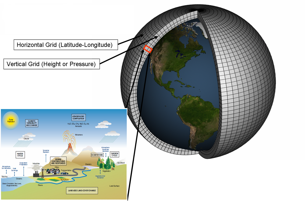
To make credible future climate projections at the regional scale, one must necessarily start from climate model simulations of the global climate system. This is because many of the processes and feedbacks that shape the response of the climate system to external forcings – imposed perturbations to the Earth's energy balance – operate and interact at the global scale. Future anthropogenic global climate change is forced primarily by emissions, and hence increasing atmospheric concentrations of GHGs and changing concentrations of aerosols. Global Climate Models (GCMs) and Earth System Models (ESMs) are computer simulations of the global climate system that can be used to make projections of future climate when driven by future scenarios of GHG and aerosol emissions. GCMs represent the physical processes and interactions (Figure 2.1a) between the atmosphere, ocean, cryosphere (ice and snow), land surface, and, in the case of ESMsFootnote 3iii, biogeochemical cycles using a numerical mathematical framework represented as a computer model.
The rate of the simulated global climate system’s response to a given scenario of anthropogenic emissions depends on the emissions themselves, but also on the way in which processes in a given GCM are represented. These two types of uncertainty – that due to assumptions about the GHG forcing scenario and that due to the climate model and our understanding of physical processes represented by the model – are two of the main sources of uncertainty that must be communicated when providing climate projections. The third source – internal variability – is, in contrast to scenario and model uncertainty, quantifiable. Internal variability is the natural, chaotic variability that we experience as weather, the occurrence of El Niño events, and so on. It is intrinsic to the coupled climate system and is an irreducible source of uncertainty.
Subsequent sections provide a brief overview on the use of climate models for making projections of global and regional climates. A link to a companion primer written for an engineering audience is provided in Appendix 2.1 (Arora and Cannon, 2018)Reference 5.
2.1.2 Model uncertainty
GCMs are based on general principles of fluid dynamics and thermodynamics, but, because of the complexity of the global climate system, they are typically run at a relatively coarse spatial discretization (e.g., grid spacing from a few tens to a few hundreds of kilometres) to be able to assess the response of the Earth’s climate to GHG changes and other radiative forcing agents. While GCMs attempt to model a range of physical, chemical, and biological processes from first principles, they can only represent our best understanding of how our planet works and how it responds to external climate forcings. The true climate system is highly complex and so it remains fundamentally impossible to model all of its processes. Numerous physical, chemical, and biological processes, typically those that operate on small spatial and temporal scales, are parameterized – which means that their effects are represented by simplified approximations – since they cannot be modelled explicitly.
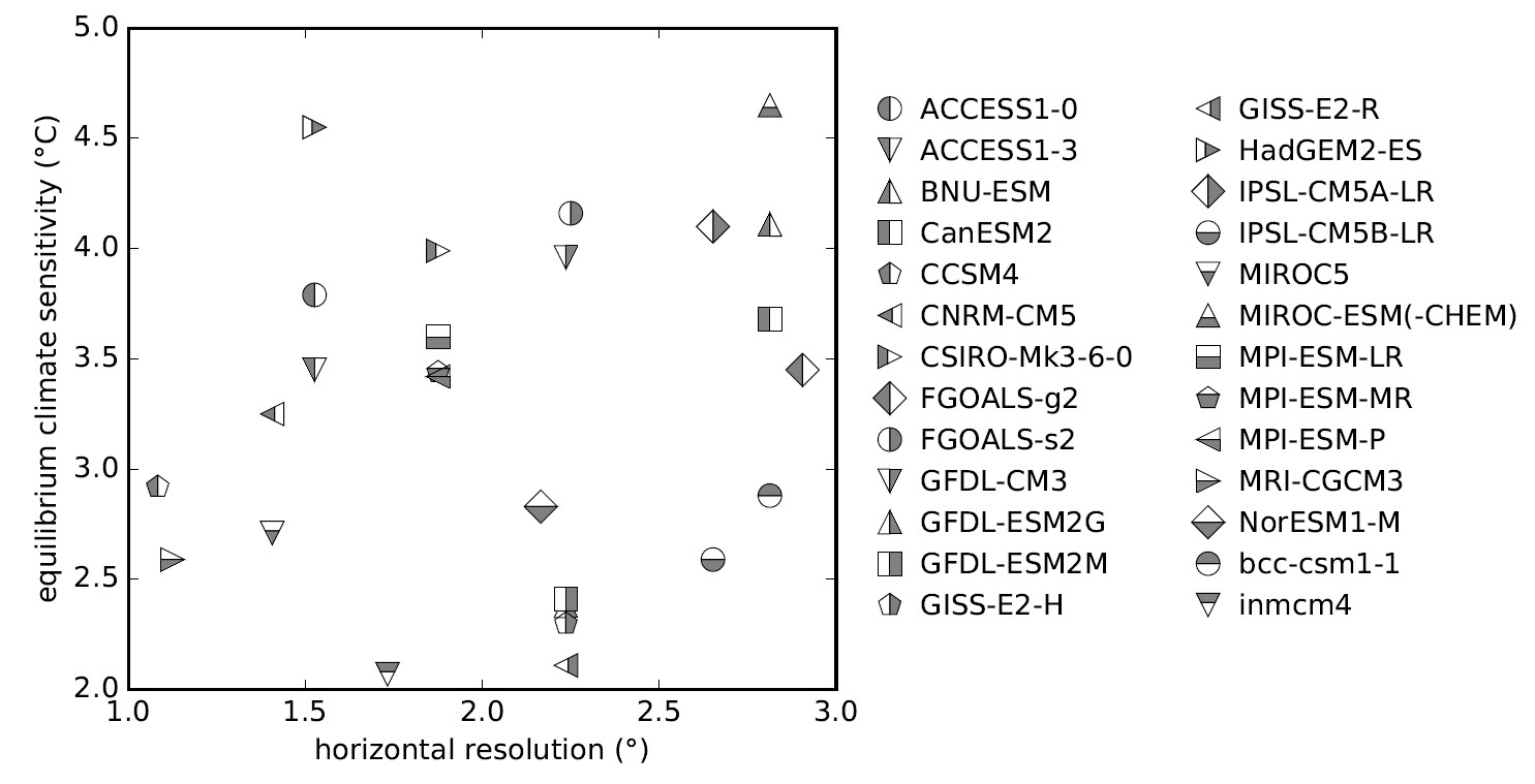
There are many climate modelling groups around the world that perform simulations with dozens of GCMs. Results are contributed to the World Climate Research Programme’s Coupled Model Intercomparison Project (CMIP; Taylor et al., 2012Reference 6; Eyring et al., 2016Reference 7). The fifth phase of CMIP (CMIP5) informed the IPCC 5th Assessment Report (IPCC, 2013)Reference 4 and a sixth phase (CMIP6) will inform the IPCC 6th Assessment Report (anticipated release, 2021-2022). While based on the same underlying principles, groups may parameterize unresolved physical processes – for example simplified representations of cloud properties and cloud microphysics – in slightly different ways and make different choices about model structure (Alexander and Easterbrook, 2015)Reference 8 and horizontal and vertical resolution. The result is that different climate models respond to the same external forcing in somewhat different ways. As an example, Figure 2.1b shows model resolution and equilibrium climate sensitivity – the long-term global mean temperature change associated with a doubling of CO2 concentration – for 26 CMIP5 climate models. Differences in cloud feedback stemming from differences in model parameterizations of cloud properties and microphysics are responsible for much of the current spread in climate sensitivity (Zelinka et al., 2017)Reference 9. While the spread in climate sensitivity is reducible in principle as our understanding of physical processes and ability to represent them in GCMs improves, the diversity among models is considered a healthy aspect of the climate modelling community and is one source of uncertainty in future climate change projections at global and regional scales.
 b)
b)
2.1.3 Scenario uncertainty
GCMs are able to simulate the response of the climate system to human induced emissions of GHGs, but cannot make predictions of future human activities. Therefore, different forcing scenarios or “pathways” of future GHG concentrations, aerosols, and land-use change must be specified as inputs to GCMs. The projections described in the IPCC 5th Assessment were based on a suite of future forcing scenarios called “Representative Concentration Pathways” (RCPs) (Van Vuuren et al., 2011)Reference 10. The RCPs were identified by approximating the radiative forcing at the end of the 21st century: RCP2.6 represents a low emission pathway (i.e., roughly compatible with the Paris Agreement) with a radiative forcing of roughly 2.6 W/m2, RCP4.5 represents modest emission mitigation pathways with a radiative forcing of roughly 4.5 W/m2, RCP6.0 an incrementally larger increase in emissions and a radiative forcing of roughly 6.0 W/m2, and RCP8.5 represents a pathway with continued growth in GHG emissions leading to a radiative forcing of roughly 8.5 W/m2 at the end of the century. For each RCP, comprehensive time series of individual greenhouse gases (CO2, CH4, N2O, CFCs, etc.), along with aerosol precursor emissions, and land-use change are provided and taken as input by GCMs, which then simulate the future response of the climate system to these external forcing scenarios, including biogeochemical feedbacksFootnote 4iv.
It is important to note that no likelihoods are ascribed to these future forcing scenarios – they are all deemed plausible, although as emissions continue to increase, low emission pathways become more difficult to achieve (e.g. Millar et al., 2017Reference 11; Raftery et al., 2017Reference 12). For instance, the low emission RCP2.6 scenario, which is consistent with limiting global temperature to roughly 2°C above preindustrial conditions, requires global carbon emissions to peak almost immediately and reduce to near zero well before the end of the century. The spread across the RCPs represents some measure of our uncertainty as to how socioeconomic factors may change in the future, particularly the extent to which emission mitigation efforts are pursued, and therefore the pace at which humans will continue to drive climate change. In order to span the range of uncertainty in future emission pathways, climate models use a range of forcing scenarios, thus providing a range of future climate projections.
2.1.4 Historical simulations and internal variability
In addition to forcing scenario simulations (e.g. from near present to 2100 under different RCPs), historical simulations provide information about past climate conditions and therefore form the baseline against which future change is compared. Historical simulations are also used to evaluate model consistency with observations of the climate system. Typically, an ensemble of 5 to 10 or more historical simulations are initialized and run based on observed historical GHG concentrations and other external climate forcings; forcing scenario simulations then continue from the end of the historical simulations. Two simulations with a given climate model that are started from different initial conditions will simulate different sequences of weather events, but it is expected that the statistics describing these events, termed the model’s climatology, will be essentially indistinguishable between simulations if the same forcing prescriptions are used. Thus, over the long historical period, each of the simulations in an ensemble of runs started from different initial conditions should show a similar increase in temperature associated with increasing concentrations of GHGs. Each historical simulation in this ensemble can thus be thought of as a plausible realization of how the historical climate could have evolved if the instantaneous state of the system in all of it details had been slightly different at the time when observations began (sometimes referred to the “butterfly effect”). A note of caution here is that none of the historical simulations can be expected to evolve in a way that matches what is seen in the observations, even if the climate model provided a perfect representation of the real climate. This is because the historical climate that we have observed is also an individual realization of the chaotic climate system. The same chaotic behaviour – variability internal to the natural climate system – underlies the roughly two-week limit on the useful horizon of instantaneous weather forecasts. The spread from a large ensemble of simulations from a single GCM and forcing scenario thus allows uncertainty due to internal variability to be evaluated.
2.1.5 Regional downscaling
When higher resolution climate scenarios are needed, one can take GCM projections and “downscale” them to higher resolution over a region of interest. Dynamical downscaling involves the use of a Regional Climate Model (RCM) – essentially a physically-based climate model that operates at higher resolution than a GCM, but over a limited-area domain (e.g., an area containing a continent such as North America or sometimes only a part of a continent). Typical grid spacings of GCMs and RCMs are around 100-250 km and 10-50 km, respectively. RCMs incorporate many of the same physical processes and parameterizations as GCMs, and indeed often share much of the same computer code. The important distinction is that RCMs are driven at their lateral boundaries by output from a GCMFootnote 5v. The regional model provides a physically-based simulation of climate within the region it covers that is consistent with the global model providing conditions at its boundaries – though it must be noted that the regional model also inherits errors and biases that may be present in the global model results.
One advantage of this two-step process in which an RCM is used to dynamically downscale a GCM is that, due to its limited area, a regional model can simulate climate on a higher-resolution grid using a similar amount of computing effort as a global model. This additional detail is often desirable, and evidence available at the time of the IPCC 5th Assessment suggests that RCMs can add value to GCM projections (Rummukainen, 2016)Reference 13 in some locations due to their better representation of topography, land/water boundaries, and certain physical processes like local feedbacks. For very high-resolution dynamical downscaling (at model resolution ≤ 4km), physical processes like atmospheric convection begin to be resolved explicitly and can lead to improved simulation of climate variables like short-duration precipitation extremes. Such convection-permitting models, however, remain largely experimental because of their very high computational costFootnote 6vi.
2.2 Constructing climate change projections
For climate change projections, the uncertainty due to model and forcing scenario spread is best addressed by not relying on climate change information from a single climate model or forcing scenario, but rather by combining results from multiple models and scenarios. For a given forcing scenario, such a multi-model ensemble samples both internal variability and model uncertainty; the relative influence of internal variability can be assessed by looking at multiple simulations from a given climate model with the same forcings. The purpose is to span the range of responses that climate models produce for a given scenario.
The relative influence of internal variability, forcing uncertainty, and model uncertainty on future climate projections depends on the variable, spatial scale, and time horizon of interest. For example, uncertainty in regional temperature projections for the near future will be dominated by internal variability (more so for regional precipitation projections), whereas projections of global mean temperature for the end of the century will be dominated by future forcing uncertainty.
To illustrate, Figure 2.2a shows time series of simulated historical and projected future global mean annual temperature anomalies, taken with respect to a 1986-2016 baseline period, for 29 CMIP5 GCMs and 3 forcing scenarios (low RCP2.6, medium RCP4.5, and high RCP8.5) for years from 1950 to 2100. Figure 2.2b shows the corresponding series of mean annual temperature anomalies for a region including Canada and adjacent waters (40°N to 75°N and 140°W to 55°W). The heavy lines indicate the multi-model average and the lighter lines indicate individual models. The high emission forcing scenario results are shown by the red lines, the medium emission scenario by the orange lines, and the low emission scenario by the blue lines; black lines show results for the historical simulations. The purple lines are for a large multi-member ensemble of a single model under the high emission scenario.
When looking at projected climate change relative to the present, the spread across models is smaller in the near term than it is toward the end of the 21st century, indicating, in part, that the effect of model uncertainty (e.g., due to differences in climate sensitivity) becomes larger the further into the future one projectsFootnote 7vii. The difference between forcing scenarios is small out to the middle of the century. This is partly because it takes some time for the Earth system to respond to prior GHG emissions (e.g., due to the large thermal capacity of the ocean), and partly because of offsetting effects of GHG and aerosol emissions in the near term (Zwiers, 2002)Reference 14. The difference between scenarios becomes large toward the end of the 21st century (as illustrated by the growing separation between the low and high emissions results). Turning to regional results for Canada, the overall pattern is similar, but overall warming and the spread in projections are both larger than at the global level. Larger warming is mostly due to Arctic amplification, which, in part, is caused by positive sea-ice albedo and snow-albedo feedbacks; melting of Arctic sea ice and reduction in Northern Hemisphere snow cover leads to more absorption of incoming solar radiation by the oceans and the land surface, which in turn enhances the initial warming. Larger spread in projections at the regional scale is mostly due to the comparatively larger amount of internal variability, reflected by the spread in the purple lines, relative to the effects of the external forcing as one moves to smaller regional scales (Deser et al., 2012)Reference 15 – variability due to internal variability is “averaged out” at the global scale.
2.3 Communicating uncertainty
In the context of projections for B&CPI climatic design variables, clear communication of each of the three sources of uncertainty is of key importance. It is common practice for information on future climate projections from multi-model ensembles, like those that contributed to CMIP5, to be provided for fixed future time periods (e.g., 2020s, 2050s, and 2080s) under different forcing scenarios. This practice combines projections from GCMs with different climate sensitivities (Figure 2.1) for each projection horizon, making it difficult to separate uncertainty due to internal variability and that due to inter-model spread (Figure 2.2).
A different approach is taken in this project. Namely, site-specific and regional projections of changes in B&CPI climatic design variables are instead provided for fixed levels of global warming (e.g., the time period associated with a +2°C change in global mean temperature). Seneviratne et al. (2016)Reference 16 showed that changes in extreme temperature and precipitation over large regions “scale” in a similar fashion with global temperature increase across forcing scenarios and models; that is, the proportional changes in these extremes are similar across scenarios and models when considered as a function of global mean temperature change. To illustrate, Figure 2.3 plots projected changes in global annual mean temperature (the data in Figure 2.2a) against changes in annual mean temperature around Canada (the data in Figure 2.2b). In this case, regional warming over Canada scales approximately linearly with changes in global mean temperature, at slightly less than twice the rate of the globe, and is roughly the same for the different forcing scenarios. Linking regional impacts to specified global warming levels – rather than to fixed time periods in which regional projections from models with different climate sensitivities (Figure 2.1) are mixed together – thus provides a convenient way to communicate climate change information. This does not lead to a reduction in uncertainty – the same information is being presented – but rather offers a straightforward way to decouple information about regional projections from information about forcing scenarios and model sensitivity. In addition, there is a direct connection with global warming targets, for example as specified under the Paris Agreement, and subsequent assessments of the likelihood of meeting such targets (Millar et al., 2017Reference 11; Raftery et al., 2017Reference 12).
2.4 Targeted research
Considering the temporal and spatial scales at which B&CPI climatic design data are required for Canada, it was deemed necessary for guidance about future climate projections to be informed by dynamically downscaled simulations from an RCM. In addition, because internal variability makes up a relatively larger component of overall climate projection uncertainty at smaller spatiotemporal scales, a large ensemble of simulations at as high a resolution as feasible was also recommended since the use of a large ensemble results in larger sample sizes from which extreme value statistics can be estimated reliably.
To meet these needs, outputs from a large 50-member ensemble of North American simulations (0.44° resolution) run by ECCC’s CCCma, some of which were sampled hourly, were used in this project. This large ensemble consists of dynamically downscaled regional simulations over North America by version 4 of CCCma’s RCM, CanRCM4, driven by global simulations from CCCma’s 2nd generation ESM, CanESM2. All 50 simulations archived 1-hr precipitation; 3-hr surface and upper air temperature; 3-hr 10m wind speed; 3-hr surface pressure; daily maximum 10m 15-min mean wind speed; daily minimum, maximum, and mean temperature; and daily mean relative humidity. In addition, 15 of the simulations archived 1-hr surface temperatures and 1-hr 10m wind speeds.
CanESM2 is a GCM with interactive atmosphere, ocean, sea ice, land, and carbon cycle components that is configured to run at ~2.8° horizontal spacing (Arora et al., 2011)Reference 17. A large initial-condition ensemble, referred to as the CanESM2 Large Ensemble (LE) (Fyfe et al., 2017)Reference 18, consisting of 50 simulations was randomly initialized starting on 1 January 1950 from the 5 historical CanESM2 ensemble members contributed by CCCma to CMIP5. Random perturbations to the initial atmospheric state at the beginning of 1950 were introduced via one of the cloud physics parameterizations. This parameterization relies on a random number generator with a pre-set seed; the 10 individual simulations split from each of the 5 CMIP5 ensemble members are based on different seeds. In this way, different historical and climate change realizations were produced without any change to the model dynamics, physics, or structure. The only differences are due to internal variability. Simulations used observed estimates of historical changes in solar, volcanic, greenhouse gas, aerosol, ozone, and land use forcings. Historical simulations end on 31 December 2005. The RCP8.5 emissions scenario was used to extend the historical simulations from January 2006 to 2100.
Regional simulations that dynamically downscale the CanESM2 LE to a 0.44° grid over North America were performed with CanRCM4 (Scinocca et al., 2016; Appendix 2.2)Reference 19. It has the same dynamical core as the Global Environmental Multiscale (GEM) model, which is an integrated numerical weather forecasting and data assimilation system developed by ECCC (Côté et al. 1998)Reference 20. CanRCM4 uses the same package of physical parameterizations as the fourth-generation Canadian Atmospheric global climate model (CanAM4) of CCCma (von Salzen et al. 2013)Reference 21, which forms the atmospheric component of CanESM2. In particular, CanRCM4 uses the deep-convection scheme of Zhang and McFarlane (1995)Reference 22, the shallow-convection scheme following von Salzen et al. (2005)Reference 23, and the Canadian Land Surface Scheme (CLASS) version 2.7 (Verseghy, 1991, 2000)Reference 24Reference 25. Appendix 2.2 provides a link to further details on the main characteristics and physical parameterizations of this RCM and its relationship with its parent global model CanESM2. A large body of literature has evaluated the ability of CanRCM4 to simulate historical climate conditions, including extreme temperature and precipitation (Diaconescu et al., 2016Reference 26; Whan and Zwiers, 2016Reference 27; Whan et al., 2016Reference 28; Whan and Zwiers, 2017Reference 29; Ben Alaya et al., 2019Reference 30), snow (Fyfe et al., 2017)Reference 18, rain-on-snow events (Jeong and Sushama, 2018b)Reference 31, extratropical cyclones (Seiler et al., 2018)Reference 32 and atmospheric rivers (Whan and Zwiers, 2016Reference 27; Tan et al., 2020Reference 33).
Climate model data used in this project are available on the Government of Canada Open Data Portal:
- The Canadian Regional Climate Model Large Ensemble
- The Canadian Earth System Model Large Ensembles
- CMIP5 multi-model ensembles of temperature projections
- CMIP5 multi-model ensembles of precipitation projections
- Statistically downscaled multi-model ensembles of mean temperature
- Statistically downscaled multi-model ensembles of maximum temperature
- Statistically downscaled multi-model ensembles of minimum temperature
- Statistically downscaled multi-model ensembles of precipitation
2.5 Guidance and recommendations
2.5.1 Model uncertainty
Projections of changes in climatic design data are computed based on CanRCM4 LE outputs at +0.5°C increments of global mean near surface air temperature change taken with respect to a historical baseline period. The choice of historical baseline involves a trade-off between including a sufficiently long record to reduce sampling uncertainty to an acceptable level, but also a short enough period to minimize the influence of climate trends on estimated design data. For reference, Kharin and Zwiers (2005)Reference 35 present an analysis of the influence of nonstationarity on extreme value analyses and Li et al. (2019a)Reference 36 assess how much climate data would be needed to reliably quantify the effects of non-stationarity on the intensity of extreme precipitation events.
To partly account for historical warming and non-stationarity of the observational record, NBCC 2015 reported observed values of temperature related climatic design elements that were updated for a 25-year period including data up to 2006. Using a similar approach, all projections here are based on a slightly longer 31-year historical baseline period spanning 1986-2016 that is representative of the most recent climate. The most commonly used period length for climatological averages is 30 years, which is the length used by the World Meteorological Organization to calculate climate normals. A simple adjustment of one year longer is adopted to avoid ambiguity in the identification of the central year in a climatological period.
Regional data are calculated based on CanRCM4 LE simulations associated with specified levels of global warming projected by CanESM2 LE under the historical and high emission RCP8.5 forcing scenario. Calculations of global mean temperature and the time of occurrence of +0.5°C to +3.5°C changes are based on 31-year periods taken with respect to this 1986-2016 baselineFootnote 8viii. Years associated with each increment thus reflect the centre year of the first 31-year period for which the average change in global mean temperature is equal to the specified warming level and for which the average change for each subsequent 31-year period relative to the base period remains above that level. The centre years of the global warming increments, as projected by CanESM2 LE with respect to the 1986-2016 baseline period, are first determined for each individual member. Median values of the central years are 2016 for +0.5°C warming (2001-2031), 2028 for +1°C warming (2013-2043), 2039 for +1.5°C warming (2024-2054), 2049 for +2°C warming (2034-2064), 2059 for +2.5°C warming (2044-2074), 2068 for +3°C warming (2053-2083), and 2077 for +3.5°C warming (2062-2092). Projections of regional changes in climatic design data from CanRCM4 LE are then based on absolute or relative differences, depending on the variable, between these 31-year future periods associated with each increment of global warming and the historical baseline period. The 25th and 75th percentiles from the available CanRCM4 LE members are also calculated to characterize uncertainty due to internal variability.
Finally, to provide information on the full range of CMIP5 model and forcing uncertainty at the global scale, the timing of the specified levels of global warming is calculated from the ensemble of available CMIP5 GCMs for the RCP2.6, RCP4.5, RCP6.0 and RCP8.5 emissions scenarios. These calculations were made by the Pacific Climate Impacts Consortium (PCIC) as part of a parallel contract with the National Research Council to support ECCC efforts in providing climatic design data for future climate states. The following description has been modified from one provided by PCIC.
It is necessary to decide which GCM runs should be used to determine when warming above a certain level has occurred. The creation of a widely accepted set of metrics of model quality is an ongoing objective of climate research where consensus on how to best separate poorer performing GCMs from better performing GCMs has not yet been achieved. It is therefore best to use as many GCMs and runs as possible to reduce the influence of model uncertainty and natural variability on results. Some GCMs, however, have only a single run while others have multiple runs. Here we choose to use a single (randomly chosen) run per GCM. The advantages of this option are that all GCMs have equal weighting and each GCM has its variability represented on an equal basis. The disadvantage of this approach is that it is technically not making use of all information available. To determine whether this disadvantage is an issue, we compared results following this option to weighting all available runs equally and found almost no difference. As a basis for selecting single runs from the full ensemble, we use the same runs that were selected for use in the IPCC AR5 Atlas (IPCC, 2013)Reference 4.
Multi-model means under all RCPs reach a global warming level of +0.5°C relative to 1986-2016 at around the same time, only a few years from present (Table 2.1). At higher warming levels the RCPs diverge from each other and multi-model means of simulations under RCPs 2.6, 4.5, and 6.0 eventually reach levels of at most +0.5°C, +1.5°C and +2°C global warming relative to 1986-2016, respectively. In the summary of the results in Table 2.1, timing is averaged together for RCPs if they reach the same level at nearly the same time (within 6 years of each other). A table with more detailed results is provided in Appendix 1.1.
Table 2.1: The year at which the indicated global mean warming ΔT relative to 1986-2016 reference period is irrevocably exceeded by the CMIP5 (single ensemble member per model) multi-model mean for RCP8.5, RCP6.0, RCP4.5, and RCP2.6 emissions scenarios. Model results are obtained from the KNMI Climate Explorer. Years are rounded to nearest year. A dash (“−”) indicates that a sustained level warming at the level specified by the corresponding ΔT does not occur before 2100 for the emissions scenario indicated. Results from different emissions scenarios are averaged together if the years when a given level of warming is reached are within 6 years of each other for the different emissions scenarios. Note that near the endpoints, the 31-year moving average window shrinks to an n-year symmetric window with n approaching 1 at the endpoint.
| ΔT | RCP 8.5 | RCP 6.0 | RCP 4.5 | RCP 2.6 |
|---|---|---|---|---|
| +0.5°C | 2023 | |||
| +1.0°C | 2035 | 2046 | — | |
| +1.5°C | 2047 | 2070 | — | |
| +2.0°C | 2059 | 2087 | — | — |
| +2.5°C | 2069 | — | — | — |
| +3.0°C | 2080 | — | — | — |
| +3.5°C | 2090 | — | — | — |
This approach – providing regional projections based on CanRCM4 LE and the timing of global warming from a multi-model, multi-scenario ensemble of GCMs – assumes that climate projection uncertainty can be partitioned into three sources, one operating primarily at the regional scale – internal variability estimated from CanRCM4 LE – and two on global scales – model uncertainty and forcing uncertainty in global warming, estimated, respectively, from the CMIP5 inter-model spread and the four emission scenarios.
Information on regional changes in climatic design data is thus decoupled from information on timing of global warming, which depends on forcing scenario and GCM sensitivity. The main assumptions of this approach are: (1) that the CanESM2-CanRCM4 LE modelling system provides an accurate estimate of the internal variability of the climate system and its regional characteristics; (2) that forcing and model uncertainty are primarily expressed in terms of the timing of global mean temperature change and not in the regional impacts of that level of warming on Canada; and (3) that the expression of regional change for a given level of global mean temperature change does not depend on the forcing scenario, i.e., how a given level of global mean temperature change is reached.
At the global scale, CMIP5 model variability compares well with observed variability at a variety of time scales (Jones et al., 2013)Reference 37. Furthermore, CanESM2 LE consistency with observed internal variability has been verified for Arctic sea ice extent (Kirchmeier-Young et al., 2017)Reference 38, snowpack in western North America (Fyfe et al., 2017)Reference 18 and atmospheric rivers affecting Canada’s west coast (Tan et al., 2020)Reference 33, amongst others.
It should be noted, however, that while relating regional change to levels of global warming reduces the influence of model uncertainty due to differences in GCM sensitivity at the global scale, the regional response may still be somewhat model-dependent. The spread in annual temperature change over Canada for a given level of global warming under the high emission scenario, shown in Figure 2.2 and Figure 2.3, is due entirely to internal variability for CanESM2 LE, but is due to both model uncertainty and internal variability for the CMIP5 GCMs. If the magnitudes of internal variability sampled by the CMIP5 RCP8.5 and CanESM2 LE RCP8.5 ensembles were the same, then model-independence of the regional response would imply that average spread should be the same for the two ensembles. For this particular variable, spread of CanESM2 LE is ~80% that of the full CMIP5 ensemble suggesting that the influence of model uncertainty is not entirely eliminated when relating regional change to global warming levels. The dependency of the strength of the influence of model uncertainty in different variables and regions of interest remains mostly untested here.
Scenario-independence of the regional climate response to levels of global warming (e.g., as indicated by the equality of global-regional temperature scaling in Figure 2.3 for different forcing scenarios) has been evaluated for temperature and precipitation extremes by Pendergrass et al. (2015)Reference 39 and Wang et al. (2017)Reference 40. Over North America, which does not have anomalously large aerosol loadings relative to other regions (e.g., in contrast with south Asia), there is little evidence to suggest that the relationship between global warming and regional changes differs between forcing scenarios.
The decoupling of regional changes from the timing of global warming means that estimates of the timing of global mean temperature change can be updated as new science emerges, for example as new GCM projections are released under CMIP6 (Eyring et al., 2016)Reference 7. Further, estimates of the regional impacts of a specified level of warming on Canada can be undertaken separately.
2.5.2 Selection of time horizons and linkage with global warming levels
For B&CPI design purposes, guidance is needed to help select the appropriate climatic design data within a given time horizon, for example 50-years for buildings (NBCC Table C-2) and 75-years for bridges (CHBDC Annex A3.1). Based on the approach adopted here for communicating projected changes in climatic design data, this means identifying the appropriate level of global warming to match the specified time horizon (Table 2.1). Once the level of global warming has been identified, one can consult chapter 3, chapter 4, chapter 5 and chapter 6 as appropriate for assessments of the projected changes in the relevant climatic design data. Location specific projections of design value changes are tabulated in Appendix 1.2, with the caveat that these should only be consulted after carefully considering the assessments in the chapters that follow.
As this is not a simple climate science question, further discussion is warranted and recommendations are left to the appropriate codes and standards bodies. Based on the information presented in this chapter on projections of global warming by the CMIP5 ensemble, however, the following preliminary recommendations are provided:
-
For the 50-year horizon, it is recommended that a warming level associated with the RCP8.5 scenario (+2.5°C) be used since the incremental change in design data relative to those for RCP4.5 or RCP6.0 is not large for this time frame;
-
For the 75-year time horizon, selection of an appropriate scenario is more complicated because the difference between different scenarios near the end of the century can be quite large. In this case, a judgement must be made on which scenario to target. Consultation with experts to assess the probability of different forcing scenarios may be needed to arrive at a final decision.
Regardless of time horizon, it may be useful to consider the projected direction of change of different types of loads. Some loads, such as snow loads are projected to decrease under all warming scenarios, and thus a conservative approach would be to base designs on current climatic design data for those elements. In contrast, other loads, such as summer thermal loads, are projected to increase, and in those cases, a conservative approach would be to use projected future design data.
A conservative choice for a long time horizon that attempts to avoid risk associated with the underestimation of loads would be to use the RCP8.5 scenario (+3.5°C) for loads that are projected to increase and to use current climatic design data for loads that are projected to decrease, acknowledging that this could lead to more expensive designs.
A compromise approach for increasing loads might be to use design data no smaller than those appropriate for a 50-year time horizon under the RCP8.5 scenario, which would imply using design data for +2.5°C warming, the level that occurs under RCP8.5 in 2069. Such a design could be expected to continue to perform well at least to the end of this century under lower emissions scenarios, such as RCP6.0, for which global warming levels are not projected to consistently exceed 2.5°C in this century. Consideration of whether the cost-efficient adaptation of a structure to future load changes will be possible would help to mitigate the risk that loads might eventually be greater than projected under RCP6.0.
Further complicating the consideration of future risks and loads is that confidence in projections of the direction and magnitude of climatic design value changes varies greatly between different design elements, with confidence being especially low for elements that are important for the determination of structural loads (snow, ice and wind loads). In contrast, confidence is relatively high in the case of temperature related elements that are important for determining future thermal loads, and is intermediate for elements that are important for the management of water and moisture in and around structures. Thus, different approaches for assessing the potential loads and risks that may arise from future climatic conditions may be needed to inform the design of the different component systems that comprise a structure.
2.6 Example – Mean Annual Temperature
2.6.1 Background
While the scope of this report is limited to guidance about future projections of climatic design data referenced in the NBCC and CHBDC, mean annual temperature is a key indicator of the climate response to human emissions of GHGs, as higher GHG concentrations result in a warmer lower atmosphere (Bindoff et al., 2013)Reference 41. Temperature change is one of the key indicators of a changing climate, with changes in many other climate variables being tied directly or indirectly to temperature change.
For these reasons, an evaluation of mean annual temperature change in Canada is both important and offers a convenient example to demonstrate the approach used to develop guidance for the NBCC and CHBDC climatic design variables in chapter 3, chapter 4, chapter 5 and chapter 6.
For each variable, information is provided in terms of (1) an assessment of existing climate science literature; (2) targeted research undertaken as part of the project to address gaps in the literature, especially as they pertain to regional climate change in Canada; and finally (3) interpretation of the implications of projected changes for climatic design data.
In this example, each of these three components is presented for changes in mean annual temperature in Canada, along with additional description of methods, maps, and tables used to develop and convey information on projected changes and uncertainty in design variables that could be considered in future NBCC and CHBDC guidance.
2.6.2 Example - Assessment
The assessment section presents a summary of existing national and international literature assessments, and, as needed, a critical overview of other climate science literature. As mentioned in chapter 1, this report makes use of calibrated language to describe assessed levels of confidence in findings and assessed likelihood of results; this calibrated language is bolded when used in the text.
According to the CCCR (Bush and Lemmen, 2019)Reference 3, it is virtually certain that Canada’s climate has warmed and that it will warm further in the future. Observed increases in mean temperature in Canada are about twice the corresponding increases in the global mean temperature. Between 1948 and 2016, the best estimate of mean annual temperature increase is 1.7°C for Canada as a whole and 2.3°C for northern Canada. While both human activities and natural variations in the climate have contributed to the observed warming in Canada, the human factor is dominant. It is likely that more than half of the observed warming in Canada is due to the influence of human activities.
The IPCC 5th Assessment concluded that “Global mean temperatures will continue to rise over the 21st century if GHG emissions continue unabated” (IPCC, 2013, p. 1031)Reference 4. Because the components of the global climate system are interconnected, temperature change in a particular part of the world, such as Canada, is closely related to change in the global mean. Thus, there is very high confidence that temperature will also continue to increase in Canada as long as GHG increases continue. This is illustrated in Figure 2.3, which shows Canadian mean temperature change versus global mean temperature change. Consistent with observed changes, Canadian mean temperature is projected to continue to increase at roughly double the global mean rate, regardless of the forcing scenario. That is, the relationship between Canadian and global temperature change remains constant, as shown by the fact that the results from the different scenarios are all aligned. This connection between global mean and Canadian mean temperature change provides a way of estimating the implications of global change for Canada under alternative forcing scenarios and levels of global warming. In other words, change in a B&CPI relevant climate variable estimated under one forcing scenario can be scaled to approximate the change under another forcing scenario, since the ratio of Canadian to global temperature change is roughly constant. Of course, this assumes that the change in the B&CPI relevant climate variable scales directly with temperature, which may not always be the case. For example, sea level will continue to rise for centuries after global mean temperature, and thus also Canadian mean temperature, has stabilized.
Future temperatures globally and in Canada will reflect the combined effect of the response to emissions of GHGs and aerosols from human emissions and natural internal variability. Natural internal climate variability is realistically simulated by the climate models used to make projections of future climate change (Jones et al., 2013)Reference 37. This is evident in the year-to-year variability in the global and Canada-average temperature time series. In contrast, the underlying forced response, as approximated by the multi-model average, is a monotonically increasing value that closely tracks the cumulative emissions of GHGs since the pre-industrial era (Allen et al., 2009Reference 42; Matthews et al., 2009Reference 43). The combination of natural variability and the slow forced response is illustrated in Figure 2.2. In assessing the impacts of a warming climate on Canada, this combination of slow forced change and natural internal variability is important to keep in mind — the future will continue to have extreme warm and cold periods superimposed on a slow warming forced by human activities.
Annual mean temperature is projected to increase everywhere in Canada, with much larger changes in northern Canada. According to the CCCR (Bush and Lemmen, 2019)Reference 3, a low emissions scenario (RCP2.6), generally compatible with the global warming limit in the Paris Agreement, will increase annual mean temperature in Canada by a further 1.8°C by mid-century (from the baseline period of 1986-2005 used by Bush and Lemmen, 2019), with temperatures remaining roughly constant thereafter. A high emissions scenario (RCP8.5), under which only limited emission reductions are realized, would see Canada’s annual mean temperature increase by more than 6°C by the late 21st century. In all cases, northern Canada is projected to warm more than southern Canada. In the near term (2031-2050), the differences in the pattern and magnitude of warming between the low emissions scenario (RCP2.6) and the high emissions scenario (RCP8.5) are modest (on the order of 0.5°C to 1°C). However, for the late century (2081-2100), the differences become very large. Under the high emissions scenario, projected temperature increases are roughly 4°C higher, when averaged for Canada as a whole, than under the low emissions scenario. The differences are even greater in northern Canada. Enhanced warming at higher latitudes is evident in the annual mean. This is a robust feature of climate projections, both for Canada and the Earth, and is due to a combination of factors, including reductions in snow and ice (which reduce albedo and thus increase solar energy absorption at the surface) and increased heat transport from southern latitudes.
2.6.3 Example - Targeted research
The targeted research section describes research and associated model analyses carried out as part of the project to address gaps in the assessed literature for a given climatic design variable.
The CCCR (Bush and Lemmen, 2019)Reference 3 provides maps of projected near term and late century annual mean temperature change for Canada based on an ensemble of 29 GCMs under low and high emission scenarios. As described in chapter 1, the approach recommended for B&CPI is instead to provide site-specific and regional changes tied to fixed levels of global warming, rather than for fixed time periods under different scenarios. Also, the design variables that could be considered in future NBCC and CHBDC guidance are communicated at specific locations (similar to NBCC Table C-2) and may require high temporal resolution (e.g., hourly) data to calculate. Furthermore, sources of uncertainty, including internal variability, must be evaluated to help assign levels of confidence to the future projections. For these reasons, this initial assessment relies on outputs from the 50-member CanRCM4 LE model ensemble.
For reference, site-specific and regional projections in this report are obtained from CanRCM4 LE as follows:
-
For each grid cell and level of global warming, climatic design data are estimated for a) each CanRCM4 ensemble member; and b) the ensemble as a whole - this “ensemble value” may be based on ensemble pooling (e.g., for the extreme value analyses) or taking the ensemble mean over the ensemble members (e.g., for the design temperatures).
-
For each grid cell and level of global warming, a) projected changes in each ensemble member are calculated with respect to the baseline ensemble average; and b) the projected change in the ensemble average is calculated with respect to the baseline ensemble average.
-
For each grid cell and level of global warming, the 25th and 75th percentiles are calculated from the projected ensemble member changes from step 2a.
-
For each site-specific location of interest and level of global warming, the a) ensemble average from step 2b; and b) 25th and 75th percentile values from step 3 are extracted for the nearest land grid cell.
-
Representative regional projections for the ensemble average and 25th and 75th percentiles are obtained by taking the spatial median over values from step 4 for large, provincial-scale areas in Canada.
Ensemble mean CanRCM4 LE projections of changes in annual mean temperature are shown in Figure 2.4 for the +1°C, +2°C, and +3°C levels of global warming; the time of occurrence of these global warming levels are provided in Section 2.5.1. To complement the maps of projected change, summaries of changes with increasing global warming levels from +0.5°C to +3.5°C are also calculated over large regions of Canada. To better represent the built environment and population centres that are relevant to B&CPI, regional summaries are based on projected changes interpolated to locations shown in Figure 2.5. These locations, which are similar to those in Table C-2 of NBCC, are concentrated in southern portions of each region.
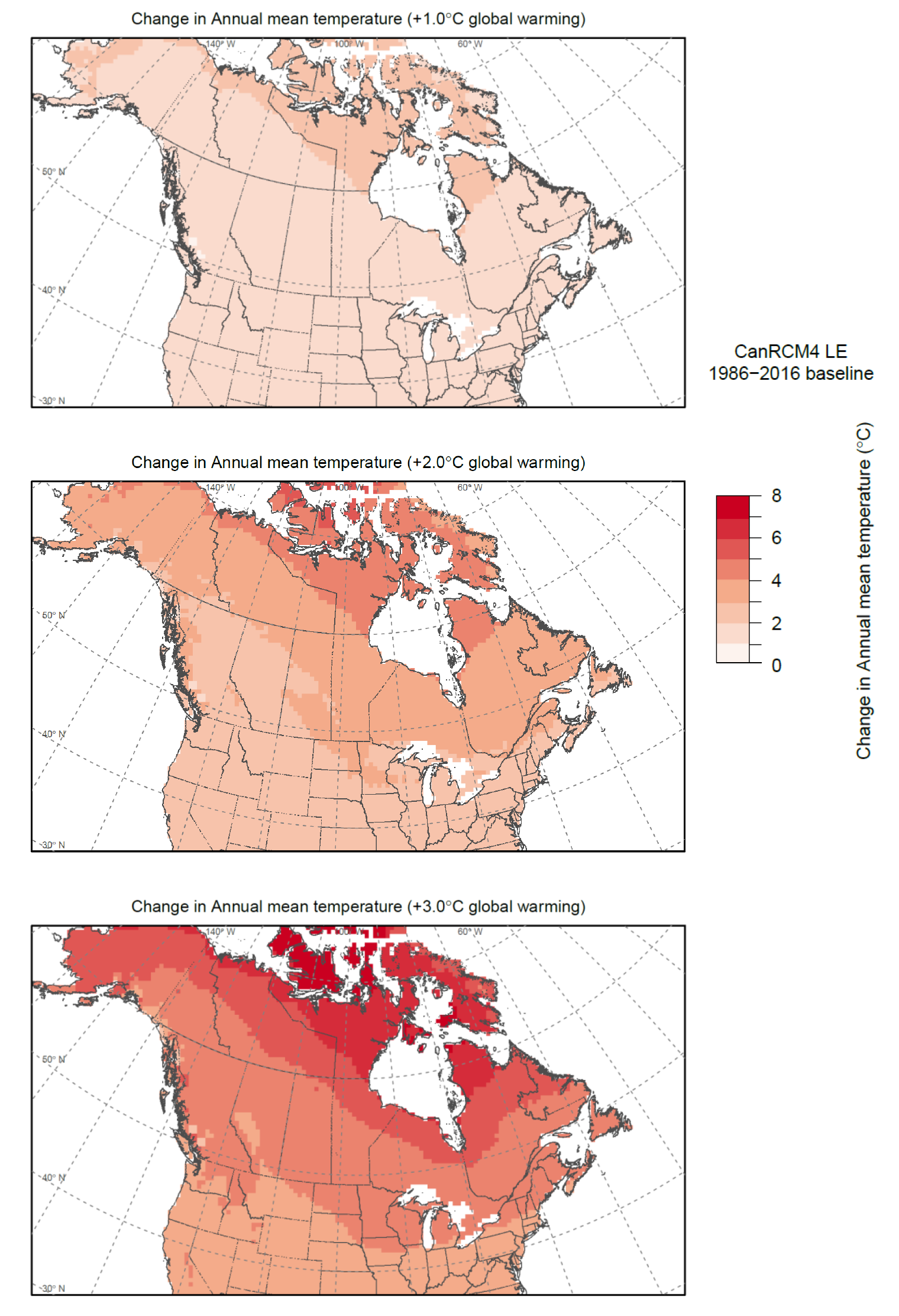
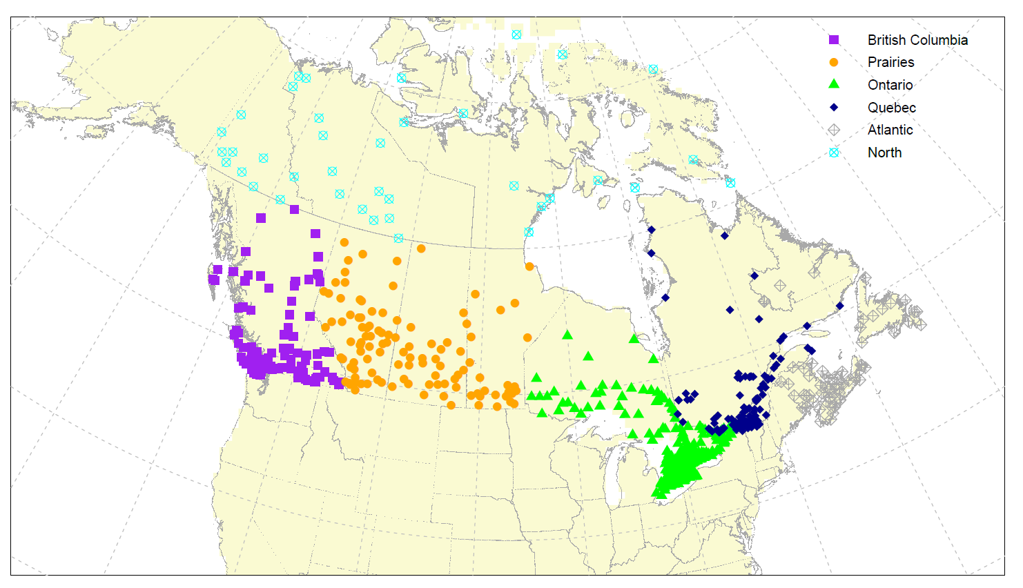
Regional summaries show median values of ensemble statistics over locations in each region (British Columbia, Prairies, Ontario, Quebec, Atlantic, and North), with internal variability communicated via the lower quartile (25th percentile) and upper quartile (75th percentile) of the CanRCM4 LE ensemble members. Regional changes in annual mean temperature are shown in Figure 2.6 and numerical summaries for the +1°C, +2°C, and +3°C global warming levels with respect to the 1986-2016 baseline period are given in Table 2.2.
Table 2.2: Projected changes in annual mean temperature for Table C-2 locations in six Canadian regions (see Figure 2.5) and Canada as a whole for +1°C, +2°C, and +3°C global warming levels with respect to the 1986-2016 baseline period. Values represent the ensemble projection (25th percentile, 75th percentile) calculated from CanRCM4 LE.
| Change in surface mean air temp. [°C] | Global warming level | ||
|---|---|---|---|
| Region | +1°C | +2°C | +3°C |
| British Columbia | 1.4 (1.3, 1.4) | 2.7 (2.6, 2.8) | 4.1 (4.0, 4.2) |
| Prairies | 1.4 (1.3, 1.6) | 2.9 (2.8, 3.1) | 4.5 (4.3, 4.5) |
| Ontario | 1.6 (1.5, 1.6) | 2.9 (2.9, 3.0) | 4.3 (4.2, 4.4) |
| Quebec | 1.6 (1.5, 1.7) | 3.1 (3.0, 3.2) | 4.6 (4.5, 4.6) |
| Atlantic | 1.5 (1.4, 1.6) | 2.8 (2.8, 2.9) | 4.2 (4.1, 4.3) |
| North | 1.9 (1.8, 2.0) | 3.7 (3.6, 3.8) | 5.5 (5.4, 5.7) |
| Canada | 1.6 (1.5, 1.6) | 3.0 (2.9, 3.0) | 4.3 (4.3, 4.4) |
Results from CanRCM4 LE are consistent with those presented in the CCCR for an ensemble of CMIP5 GCMs. Canadian temperatures in each region increase proportionally with global mean temperature change, at a rate between approximately 1.5 to 2 times that of the global mean; higher sensitivity is evident in the North. The relative magnitude of the forced change to internal variability in these regional averages – the “signal-to-noise” ratio – is high, which means that regional warming is a robust signal that emerges from the noise of historical climate variability at very low levels of global mean temperature change.
2.6.4 Example - Interpretation
The interpretation section combines findings from the scientific assessment with those from the targeted research to provide guidance and recommendations on projected changes that could be considered in future NBCC and CHBDC guidance on climatic design data.
Annual mean temperature change is a Tier 1 variable. Available evidence from the CCCR (Bush and Lemmen, 2019)Reference 3 and simulations from CanESM2-CanRCM4 LE suggests that it is virtually certain that Canada’s climate will warm further in the future. Projected increases in annual mean temperature in regions of Canada at locations relevant to B&CPI are about 1.5 to 2 times the corresponding increases in the global mean temperature, with larger increases in the north. For Canada, results are consistent between CMIP5 GCMs and the CanESM2-CanRCM4 LE (Figure 2.6), and are independent of the forcing scenario (e.g., Figure 2.3).
Projected changes in annual mean temperature at locations similar to those in Table C-2 of NBCC are provided in Appendix 1.2. Because of the consistency in the different lines of evidence noted above, data are taken directly from CanRCM4 LE projections for each global warming level. The level of agreement between ensemble members – an estimate of uncertainty due to internal variabilityFootnote 9ix – is communicated in terms of the noise-to-signal ratio, the ratio of ensemble spread to the magnitude of forced change
where Δx is the projected change, σr is a robust estimate of the ensemble standard deviation (σr = IQR/1.349), and IQR is the interquartile range. Values of NS ratio are on a scale between 0 and 1 (values > 1 are set to 1).
A value of the NS ratio that is close to 0 means that the ratio of simulated internal variability to forced change is small, or, conversely, that the signal-to-noise ratio is large. An NS value equal to 1 means that the ensemble standard deviation is the same magnitude as the projected change; in other words, the signal-to-noise ratio is small. NS ratio ranges are used here in combination with an expert assessment that considers additional unquantified sources of uncertainty to help communicate the final assessed level of confidence in the projections.
It must be stressed that NS ratio values cannot be used meaningfully in isolation. For some variables, the value of the NS ratio will be close to 1 simply because the magnitude of projected change is very small. If the overall level of understanding about causes of the projected change is high, then the final assessment of confidence will likely also be high. For other variables, confidence in the model simulations may be low (e.g., due to the inability of the RCM to resolve important physical processes), irrespective of the ratio of simulated internal variability to forced change.
For annual mean temperature change, values of NS ratio for CanRCM4 LE are universally close to 0 (mean values < 0.2 for all levels of global warming). In combination with the overall strong evidence reported in national and international assessments, there is very high confidence in future projections of annual mean temperature change.
3. Temperature
3.1 Heating degree days, design temperatures, and minimum and maximum daily mean temperature
3.1.1 Assessment
Climatic design data related to surface temperature are reported in the NBCC (heating degree days and hourly design temperatures for January and July) and the CHBDC (maximum and minimum mean daily air temperatures). Changes in these variables are closely linked with those reported in chapter 2 for mean annual temperature, and hence the assessment provided there is also relevant in this chapter. Furthermore, given their seasonal nature – July hourly extremes and maximum daily mean temperatures are related to summer temperatures, and heating degree days, January hourly extremes, and minimum daily mean temperatures are related to winter temperatures – assessments of seasonal temperatures and temperature extremes are also pertinent.
According to the CCCR (Bush and Lemmen, 2019)Reference 3, seasonal mean temperatures across Canada have increased, with the greatest warming occurring in winter. This corresponds with climate change projections, which indicate that seasonal mean temperature will increase further everywhere, with much larger changes in northern Canada in winter. Future warming will be accompanied by a longer growing season, fewer heating degree days, and more cooling degree days. Extreme temperature changes, both in observations and future projections, are consistent with warming. Extreme warm temperatures have become hotter, while extreme cold temperatures have become less cold. Such changes are projected to continue in the future, with the magnitude of change generally proportional to the magnitude of mean temperature change.
In all cases, northern Canada is projected to warm more than southern Canada, and winter temperatures are projected to increase more than summer temperatures. This high-latitude amplification is not apparent in summer because Arctic Ocean surface temperatures rise only slowly, being constrained by the absorption of the latent heat of fusion as ice continues to melt and by the absorption of solar radiation by open ocean surfaces, from which heat is subsequently transferred to deeper waters. In southern Canada, projected winter temperature change is larger in the east than in the west, with British Columbia projected to warm slightly less than elsewhere in Canada. The projected summer change is more uniform across the country.
3.1.2 Targeted research
The CCCR provides maps of projected near term and late century seasonal temperature change for Canada based on an ensemble of 29 GCMs under low and high emission scenarios. Regional projections of changes in heating degree days are also provided for the same time periods, models, and emission scenarios. As described in chapter 1, the approach recommended for B&CPI is instead to communicate regional changes that are tied to fixed levels of global warming, rather than to fixed time periods under different scenarios. This approach is evaluated, in a limited manner, in an analysis of climate indices for Canada by Li et al. (2018)Reference 44. Their results for heating degree days informed both the CCCR and this report. A link to the full analysis is provided in Appendix 2.3.
Climate model simulations of the historical climate often differ somewhat from the observed climate – a reflection of model biases (Flato et al. 2013)Reference 45. These biases arise for a number of reasons, including difficulties in accurately simulating clouds and the atmospheric circulation, incomplete process understanding at unresolved scales, and an inability to resolve fine scale topographic variability. Temperature indices like heating degree days below 18°C depend on absolute thresholds, which means that biases in the climatic mean state that is simulated by the model can affect future projections. As a result, where absolute values are important, some form of bias correction may be needed. Hence, the additional research that was undertaken to assess the projected changes in heating degree days (see Li et al., 2018; Appendix 2.3)Reference 44 is based on statistically downscaled and bias-corrected CMIP5 GCM simulations.
To extend this work further for this report, future projections based on the CanESM2-CanRCM4 LE ensemble have been calculated for different global warming levels. All of the hourly and daily temperature variables required to calculate the NBCC and CHBDC temperature variables are included in the CanRCM4 LE archive, but like other models, CanRCM4 LE is also affected by biases. Thus the CanRCM4 LE simulations used here to calculate heating degree days were first bias-corrected and downscaled following Sobie and Murdock (2017)Reference 46. On the other hand, changes in indices defined in a relative sense, such as the projected changes in the 2.5th percentile of January hourly temperatures, are generally less affected by biases because the percentile threshold involved is calculated separately for observations and from the model output. Results reported for hot and cold extremes – January and July design temperatures and minimum and maximum mean daily temperatures – are therefore based on CanRCM4 LE output that has not been bias corrected, as they do not depend on the crossing of fixed thresholds, such as the 18°C used for heating degree days.
January 2.5%, January 1%, and July 2.5% dry bulb design temperatures were estimated based on simulated hourly mean near surface air temperatures from the 15 CanRCM4 LE simulations with archived hourly temperatures. Similarly, values of wet bulb temperature were calculated from hourly mean relative humidity and air temperature output following Stull (2011)Reference 47. Heating degree days below 18°C were estimated from bias corrected and downscaled versions of the simulated daily mean near surface air temperatures from all 50 CanRCM4 LE members. For hourly design temperatures, the specified design data were estimated by (1) pooling all January (or July) hourly temperatures for a given ensemble member; (2) calculating the specified percentile(s); and finally (3) taking the ensemble mean across all simulations.
CanRCM4 LE projections indicate progressively fewer heating degree days (Figure 3.1), increases in January and July design temperatures (Figure 3.2), and increases in minimum mean daily temperature and maximum mean daily temperatures (Figure 3.3) in lock-step with the change in global mean temperature. Overall, extreme warm temperatures will become hotter, while extreme cold temperatures will become less cold, with the magnitude of change generally proportional to the magnitude of global mean temperature change.
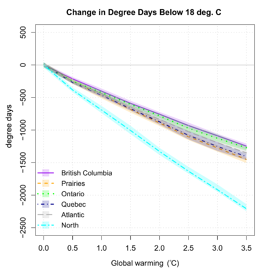
Uncertainty in these projections arises from both unforced climate variability that is intrinsic to the climate system (called internal variability) and forcing scenario and model related uncertainties. As noted in chapter 2, the internal variability can be well quantified with the CanRCM4 large ensemble, whereas the other factors contributing to the uncertainty of the projections are not easily quantified. Nevertheless, the available assessments and literature suggest that for temperature related quantities, forcing scenario uncertainty dominates these latter two sources, particularly for larger levels of warming. Further, research indicates that the approach used in this report, which references changes in design data to specified changes in global mean temperature levels, helps to reduce sensitivity to model and scenario uncertainty.
The magnitude of the climate change signal relative to internal variability can be estimated from the ensemble spread of the CanRCM4 LE simulations (see the shaded areas in Figure 3.1, Figure 3.2 and Figure 3.3). The resulting signal-to-internal-noise ratio for heating degree day projections, which integrate temperature exceedances over time, is very high, comparable to that for annual mean temperature. The signal emerges from the noise of historical internal climate variability at the +0.5°C global warming level. Forced changes in the other temperature indices emerge at similar levels of global warming, despite exhibiting larger internal variability, especially for hourly design temperatures. The 1% and 2.5% design temperatures sample extreme conditions that occur over a very small portion of each year (8 and 19 hours, respectively), and hence are subject to much larger interannual variability. There is also less confidence in the model’s ability to simulate values in the extreme upper and lower tails well, because the feedback processes that allow such values to occur might not be well represented. Similarly, the annual minimum and annual maximum daily mean temperatures depend on the single most extreme cold and hot days in a year. For reference, regional summaries of projected changes and ensemble spread are provided in Table 3.1, Table 3.2, Table 3.3 and Table 3.4.
Table 3.1: Projected changes in heating degree days below 18°C for locations approximating Table C-2 locations in six Canadian regions and Canada as a whole for +1°C, +2°C, and +3°C global warming levels with respect to the 1986-2016 baseline period. Values represent the ensemble projection (25th percentile, 75th percentile) calculated from bias corrected CanRCM4 LE simulations.
| Change in degree days below 18°C [°C days] | Global warming level | ||
|---|---|---|---|
| Region | +1°C | +2°C | +3°C |
| British Columbia | -403 (-447, -363) | -757 (-808, -722) | -1088 (-1128, -1057) |
| Prairies | -461 (-515, -428) | -891 (-938, -845) | -1274 (-1332, -1235) |
| Ontario | -424 (-461, -393) | -781 (-820, -746) | -1127 (-1178, -1068) |
| Quebec | -466 (-494, -430) | -874 (-917, -825) | -1252 (-1321, -1183) |
| Atlantic | -456 (-489, -420) | -834 (-861, -795) | -1194 (-1258, -1127) |
| North | -692 (-740, -629) | -1328 (-1328, -1274) | -1917 (-1947, -1835) |
| Canada | -449 (-487, -411) | -836 (-887, -794) | -1196 (-1257, -1139) |
Table 3.2: Projected changes in January 2.5% design temperature (top) and January 1% design temperature (bottom) for locations approximating Table C-2 locations in six Canadian regions and Canada as a whole for +1°C, +2°C, and +3°C global warming levels with respect to the 1986-2016 baseline period. Values represent the ensemble projection (25th percentile, 75th percentile) calculated from CanRCM4 LE.
| Change in January 2.5% design temp. [°C] | Global warming level | ||
|---|---|---|---|
| Region | +1°C | +2°C | +3°C |
| British Columbia | 2.3 (1.4, 3.3) | 4.9 (3.5, 6.6) | 6.7 (5.0, 8.8) |
| Prairies | 2.9 (1.8, 4.1) | 5.2 (3.3, 6.7) | 8.1 (6.3, 10.1) |
| Ontario | 4.1 (3.4, 4.7) | 6.9 (6.0, 7.6) | 10.1 (9.3, 11.3) |
| Quebec | 4.3 (3.4, 5.2) | 7.6 (6.9, 8.3) | 11.3 (10.3, 12.1) |
| Atlantic | 4.1 (3.5, 4.6) | 7.1 (6.5, 7.5) | 10.1 (9.4, 10.9) |
| North | 3.3 (2.7, 4.0) | 6.2 (5.3, 7.0) | 9.5 (8.4, 10.4) |
| Canada | 3.6 (3.0, 4.4) | 6.2 (5.5, 7.3) | 9.4 (8.6, 10.8) |
| Change in January 1% design temp. [°C] | Global warming level | ||
|---|---|---|---|
| Region | +1°C | +2°C | +3°C |
| British Columbia | 2.3 (1.3, 3.4) | 5.0 (3.4, 6.8) | 6.9 (5.0, 8.9) |
| Prairies | 2.7 (1.5, 4.1) | 5.0 (3.1, 6.6) | 8.1 (6.3, 9.8) |
| Ontario | 4.2 (3.3, 5.0) | 7.1 (6.3, 8.1) | 10.8 (9.6, 12.2) |
| Quebec | 4.3 (3.1, 5.2) | 7.7 (6.7, 8.2) | 11.7 (10.5, 12.5) |
| Atlantic | 4.0 (3.3, 4.8) | 7.5 (6.8, 8.1) | 10.9 (10.1, 11.4) |
| North | 3.2 (2.4, 4.0) | 6.3 (5.0, 7.0) | 9.1 (7.9, 10.4) |
| Canada | 3.8 (3.0, 4.6) | 6.5 (5.7, 7.6) | 9.8 (8.5, 11.1) |
Table 3.3: Projected changes in July 2.5% dry bulb design temperature (top) and July 2.5% wet bulb design temperature (bottom) for locations approximating Table C-2 locations in six Canadian regions and Canada as a whole for +1°C, +2°C, and +3°C global warming levels with respect to the 1986-2016 baseline period. Values represent the ensemble projection (25th percentile, 75th percentile) calculated from CanRCM4 LE.
| Change in July 2.5% dry design temp. [°C] | Global warming level | ||
|---|---|---|---|
| Region | +1°C | +2°C | +3°C |
| British Columbia | 2.2 (1.8, 2.6) | 4.2 (3.7, 4.8) | 6.8 (6.2, 7.4) |
| Prairies | 2.3 (1.6, 2.7) | 4.0 (3.4, 4.7) | 6.0 (5.4, 6.5) |
| Ontario | 1.6 (1.3, 1.9) | 3.0 (2.5, 3.4) | 4.1 (3.8, 4.5) |
| Quebec | 1.4 (1.1, 1.7) | 3.0 (2.7, 3.3) | 4.1 (3.9, 4.5) |
| Atlantic | 1.3 (1.1, 1.6) | 2.8 (2.6, 3.0) | 4.1 (3.9, 4.4) |
| North | 1.7 (1.3, 2.2) | 3.2 (2.7, 3.8) | 4.7 (4.3, 5.3) |
| Canada | 1.6 (1.3, 1.9) | 3.0 (2.7, 3.5) | 4.3 (4.0, 4.6) |
| Change in July 2.5% wet design temp. [°C] | Global warming level | ||
|---|---|---|---|
| Region | +1°C | +2°C | +3°C |
| British Columbia | 1.8 (1.5, 2.1) | 3.5 (3.2, 3.8) | 5.3 (5.0, 5.8) |
| Prairies | 1.8 (1.3, 2.0) | 3.1 (2.8, 3.4) | 4.6 (4.3, 4.9) |
| Ontario | 1.2 (1.0, 1.4) | 2.3 (2.1, 2.6) | 3.2 (3.1, 3.4) |
| Quebec | 1.1 (0.9, 1.4) | 2.4 (2.2, 2.5) | 3.3 (3.1, 3.5) |
| Atlantic | 1.3 (1.2, 1.4) | 2.6 (2.4, 2.7) | 3.8 (3.6, 3.9) |
| North | 1.6 (1.3, 1.9) | 2.8 (2.5, 3.3) | 4.3 (4.0, 4.8) |
| Canada | 1.3 (1.1, 1.5) | 2.5 (2.2, 2.7) | 3.6 (3.3, 3.8) |
Table 3.4: Projected changes in annual maximum daily mean temperature (top) and annual minimum daily mean temperature (bottom) for locations approximating Table C-2 locations in six Canadian regions and Canada as a whole for +1°C, +2°C, and +3°C global warming levels with respect to the 1986-2016 baseline period. Values represent the ensemble projection (25th percentile, 75th percentile) calculated from CanRCM4 LE.
| Change in max. mean temp. [°C] | Global warming level | ||
|---|---|---|---|
| Region | +1°C | +2°C | +3°C |
| British Columbia | 1.7 (1.4, 2.1) | 3.6 (3.2, 4.0) | 5.6 (5.2, 6.0) |
| Prairies | 1.8 (1.4, 2.2) | 3.5 (3.1, 3.9) | 5.2 (4.8, 5.6) |
| Ontario | 1.5 (1.2, 1.7) | 2.7 (2.4, 2.9) | 3.9 (3.5, 4.2) |
| Quebec | 1.4 (1.1, 1.7) | 2.6 (2.3, 2.9) | 3.8 (3.6, 4.2) |
| Atlantic | 1.4 (1.2, 1.6) | 2.6 (2.4, 2.8) | 3.9 (3.7, 4.2) |
| North | 1.5 (1.2, 1.9) | 2.9 (2.6, 3.3) | 4.4 (4.1, 4.8) |
| Canada | 1.5 (1.2, 1.8) | 2.7 (2.4, 3.0) | 4.0 (3.7, 4.3) |
| Change in min. mean temp. [°C] | Global warming level | ||
|---|---|---|---|
| Region | +1°C | +2°C | +3°C |
| British Columbia | 2.2 (1.6, 2.8) | 4.3 (3.6, 5.1) | 6.5 (5.6, 7.2) |
| Prairies | 2.6 (1.9, 3.3) | 5.3 (4.4, 6.0) | 8.0 (7.2, 8.8) |
| Ontario | 3.2 (2.6, 3.8) | 6.5 (6.0, 7.0) | 9.4 (9.0, 9.9) |
| Quebec | 3.8 (3.2, 4.4) | 7.6 (6.9, 8.2) | 11.1 (10.4, 11.7) |
| Atlantic | 3.6 (3.0, 4.0) | 7.1 (6.6, 7.5) | 9.8 (9.2, 10.3) |
| North | 2.9 (2.2, 3.5) | 5.8 (5.2, 6.5) | 9.1 (8.4, 9.9) |
| Canada | 3.0 (2.5, 3.5) | 5.9 (5.4, 6.5) | 9.0 (8.4, 9.6) |
Spatially, regional patterns of warming in the NBCC and CHBDC temperature variables (Figure 3.4, Figure 3.5, Figure 3.6, and Figure 3.7) generally mirror those projected for seasonal mean temperatures: winter variables (cold extremes) experience larger warming in the north, whereas summer variables (hot extremes) warm fastest in southwestern Canada. When compared with seasonal projections reported in the CCCR (Bush and Lemmen, 2019)Reference 3, July design temperatures are projected to track the projected changes in summer mean temperature, but at a higher rate. Similarly, January design temperatures are projected to warm faster than winter mean temperature. A similar pattern of change is seen for maximum daily mean temperature and minimum mean daily temperature. Regionally, there is some evidence of enhanced warming over mountainous regions due to local snow albedo feedbacks (Walton et al., 2017)Reference 48.
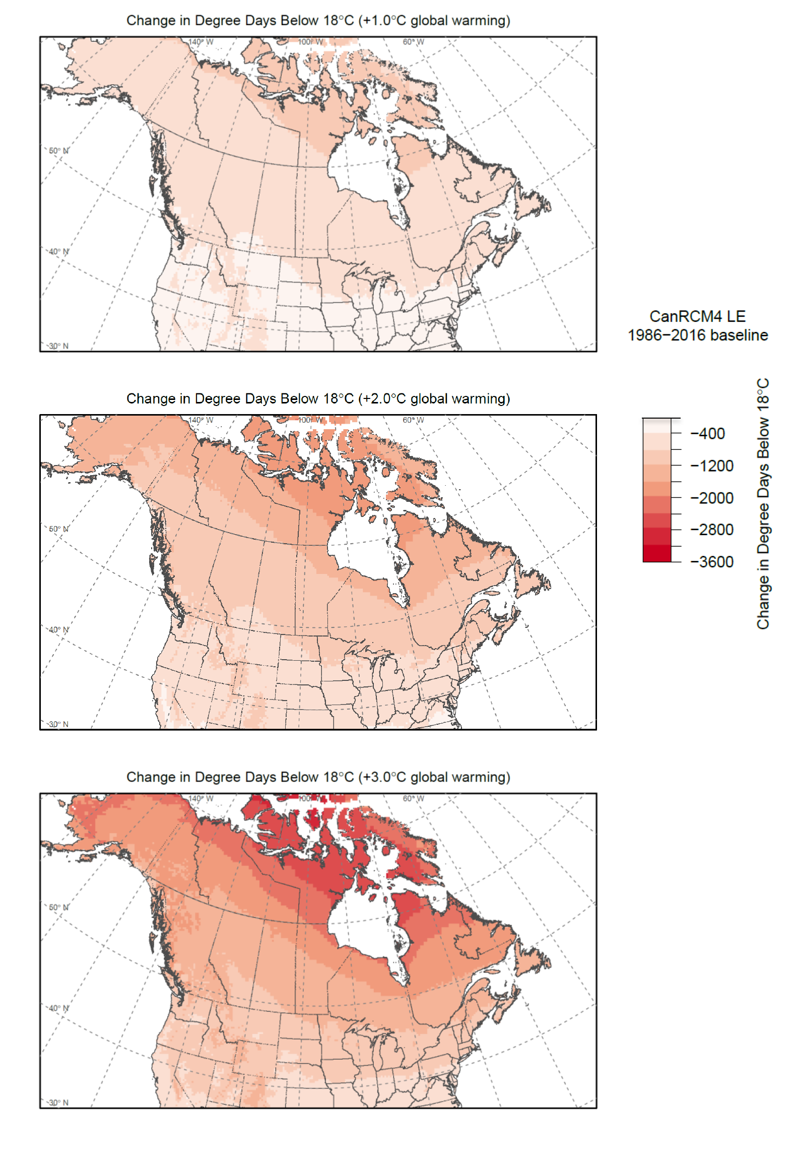
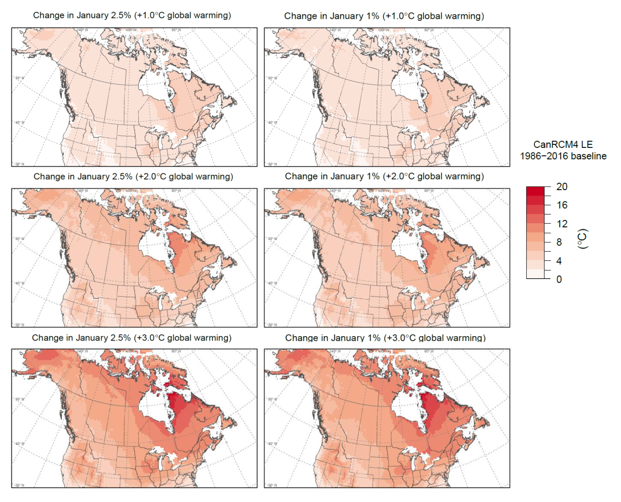
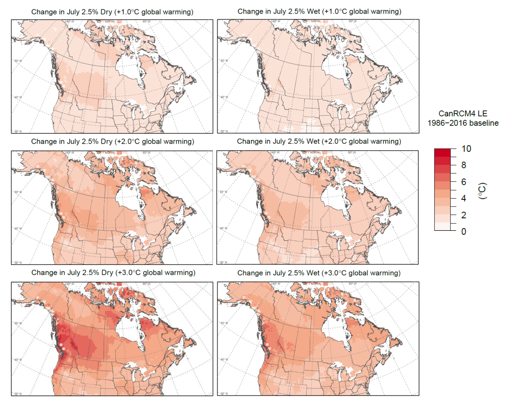
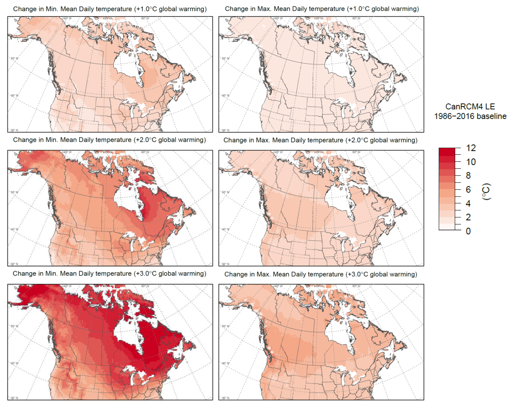
Results are generally consistent with those projected by CMIP5 GCMs. For heating degree days and indices related to temperature extremes, projections by different climate models (Appendix 2.3) for the near term (2031-2050) under a high emission scenario (RCP8.5) agree on the direction (increasing or decreasing) of changes for almost all regions. The model projections for the late century (2081-2100) also agree on the direction of changes for all temperature variables for every region under a high emission scenario (RCP8.5). This indicates the robustness of projected changes in temperature variables for the future.
3.1.3 Interpretation
NBCC and CHBDC climatic design data related to surface temperature are Tier 1 variables. In accordance with projections for annual mean temperature (chapter 2), available evidence from the CCCR (Bush and Lemmen, 2019)Reference 3, simulations from CMIP5 GCMs, and simulations from CanESM2-CanRCM4 LE are consistent and indicate that the warming of Canada’s climate (virtually certain) will lead to increases in January and July design temperatures and minimum and maximum mean daily temperatures, and decreases in heating degree days in all regions of Canada. Spatially, climatic design data that describe the cold part of the year tend to change more as one moves from south to north, whereas changes in hot extremes are more spatially uniform. In general, projected changes in temperature extremes scale roughly linearly with global warming at a rate that exceeds that for annual mean temperature.
Projected changes in surface temperature indices at locations approximating Table C-2 locations are provided in Appendix 1.2. It is not possible to attach a level of confidence to these individual place specific projections, but confidence is necessarily lower than for the regional assessments of projected changes in temperature related design data. This is because the limitations of local process representation in CanRCM4 and its constituent land surface model can be expected to compound and exacerbate any biases and errors that are apparent on larger scales.
As was the case for annual mean temperature, values are calculated from CanRCM4 LE projections for each global warming level. In general, the level of agreement between ensemble members, which are different because each is affected by its own, independent, realization of internal variability, is moderate to high at regional scales. The warming level (and hence time; see Table 2.1) at which changes emerge from the noise of internal variability can be assessed by considering values of NS ratio. For temperature related design variables, values of NS ratio < 0.2 are reached at the majority of locations at global warming levels of +0.5°C (heating degree days), +1.0°C (July 2.5% wet bulb design temperature), +1.5°C (minimum and maximum mean daily temperatures, January 2.5% design temperature, and July 2.5% dry bulb design temperature), and +2.0°C (January 1% design temperature). Given the convergence of evidence from international and national assessments and different climate models, there is high confidence in future projections of climatic design data related to surface temperature at regional scales. Relative to projections of annual mean temperature, for which there is very high confidence, there is somewhat greater uncertainty for projections of temperature related design data due to higher internal variability, the influence of model bias on exceedances of absolute thresholds as in the case of heating degree days and uncertainties associated with the associated downscaling and bias adjustments, and higher uncertainty in climate model performance for extremes. As noted in the previous paragraph, confidence in projections at individual locations is necessarily lower, even if values of the NS ratio are small, since there is lower confidence that the local details of the simulation of temperature are well represented in CanRCM4 (and for that matter, all other models operating at comparable or lower spatial resolutions).
4. Precipitation and moisture
4.1 Annual total precipitation and rainfall
4.1.1 Assessment
The assessment of historical trends and future projections of precipitation in the CCCR (Bush and Lemmen, 2019)Reference 3 concluded that there is medium confidence that annual mean precipitation has increased, on average, in Canada, with larger percentage increases in northern Canada. Such increases are consistent with model simulations of anthropogenic climate change. Annual total precipitation is projected to increase everywhere in Canada over the 21st century, with larger percentage changes in northern Canada and in mountainous areas of western Canada. Since the amount of precipitation is low in the Arctic, even modest changes in absolute amount translate into large percentage changes in the North. As temperatures increase with global warming, there will be a continued shift from snow to rain. Hence, the proportion of annual total precipitation falling as rain is also projected to increase across Canada.
In relative terms, the effect of global warming on precipitation is weaker relative to its natural unforced variability (the so-called internal variability) than for temperature. Thus, the estimation of changes in precipitation is substantially more uncertain. Precipitation changes are also affected by orography, proximity to moisture sources such as water bodies, atmospheric circulation changes, and interactions with the land surface that influence changes in local water balances, and thus they exhibit more regional variation than changes in temperature.
Projection results for regional precipitation are similarly affected, and thus have lower confidence than projection results for temperature. Projection results for precipitation are also thought to be much more strongly influenced by model uncertainties than for temperature. These sources of model uncertainty include incomplete understanding of precipitation producing processes and the effects of biases in other aspects of the representation of the climate. Limitations associated with the spatial resolutions of most global and regional climate models are also of great concern as these dictate the need to use approximations to represent the effects of sub-grid scale processes such as convection and to use smoothed representations of the surface orography that remove many small-scale details that are important for local precipitation production. The multi-model spread in projections is therefore substantially higher in precipitation projections, consistent with both lower signal-to-internal-noise ratios and large, but difficult to quantify, uncertainties in the model representation of the physical processes that produce precipitation.
Results for projected changes in total precipitation from the CanESM2-CanRCM4 LE are consistent with the IPCC 5th Assessment (IPCC, 2013)Reference 4, in that the high latitudes are projected to experience a large relative increase in annual total precipitation by the late 21st century under the high emission (RCP8.5) scenario. This high latitude increase is a common feature of multiple generations of climate models and can be explained by the expected warming-induced large increase in the poleward transport of atmospheric water vapour by the atmospheric circulation. These model simulated changes correspond with observed changes in that an increase in annual total precipitation observed in the high latitudes over the historical period has been detected and can be attributed to human influence (Min et al., 2008Reference 49; Wan et al., 2015Reference 50). Based on these findings, there is high confidence that annual precipitation and rainfall will increase in Canada with global warming. Due to higher internal variability relative to temperature and much more evidence that model uncertainty contributes to overall projection uncertainty, there is low to medium confidence in more detailed regional projections.
4.1.2 Targeted research
The CCCR (Bush and Lemmen, 2019)Reference 3 provides maps of projected near term and late century annual precipitation change for Canada based on an ensemble of 29 GCMs under low and high emission scenarios. Regional projections of changes in annual total precipitation are also summarized for the same time periods, models, and emission scenarios. As described in chapter 1, the approach recommended for B&CPI is instead to communicate regional changes that are tied to fixed levels of global warming, rather than to fixed time periods under different scenarios. This approach is evaluated in an analysis of climate indices for Canada by Li et al. (2018)Reference 44, who found that projections of precipitation from CMIP5 models do not fully agree on the sign of changes in most Canadian regions at a global warming level of approximately +2°C with respect to the preindustrial period, but they did fully agree at +4.5°C, consistent with the strengthening of the signal in projected precipitation change as warming progresses. These results, which are subject to all of the uncertainties discussed in section 4.1.1, have informed both the CCCR and this report; a link to the full analysis is provided in Appendix 2.3.
To extend this work, future projections of annual precipitation and annual rainfall based on the CanESM2-CanRCM4 LE ensemble have been calculated for different global warming levels. Annual rainfall is inferred from the difference between the diagnosed total precipitation and snowfall flux variables. Bias adjustments were not made for this analysis because the focus here is on relative changes in precipitation and rainfall rather than absolute changes. Consistent with results from CMIP5 simulations, CanRCM4 LE projects annual precipitation to increase everywhere in Canada over the 21st century, with larger percentage changes in northern Canada (Figure 4.1). Annual rainfall is also projected to increase, especially in the Arctic and over mountainous areas of western Canada, although we have considerably lower confidence in these regional variations given that projected changes in rainfall were not assessed in IPCC (2013)Reference 4. Regionally, relative changes in both annual precipitation and annual rainfall scale approximately linearly with global warming. Increases in rainfall involve two components, one due to increases in atmospheric moisture caused by warming and the other due to the shift from snow to rain due to warming. In most regions, annual rainfall is projected to increase at slightly less than double the rate of annual precipitation; greater intensification of rainfall is seen in the North and British Columbia (Figure 4.2).
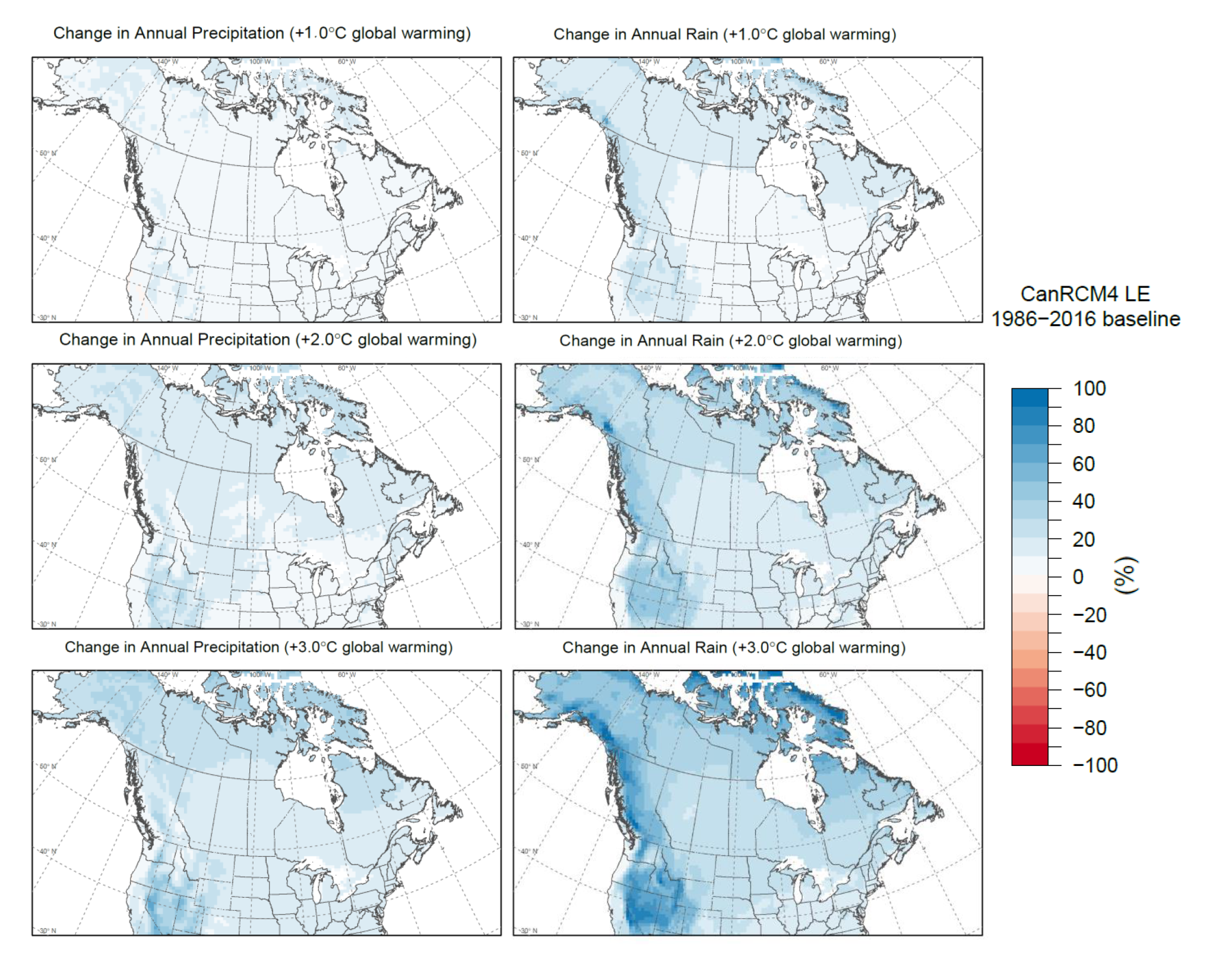
For reference, numerical summaries of projections made with CanRCM4 for the +1°C, +2°C, and +3°C global warming levels are given in Table 4.1. While the signal-to-internal-noise ratio of forced changes in precipitation and rainfall is smaller than for annual temperature (chapter 2), the central half of the ensemble members agree on the sign of projected changes in both annual precipitation and annual rainfall in all regions at all global warming levels. If one considers the full CanRCM4 LE spread (i.e., extending beyond just the interquartile range) at +1°C global warming from the 1986-2016 baseline, which is roughly equivalent to +2°C from preindustrial, in 5 of the 6 regions all members project regional increases in both annual precipitation and annual rainfall. Further, just 2 members in Ontario project decreases in annual precipitation. Thus, at these scales, the forced signals in both annual precipitation and annual rainfall are sufficiently strong at this level of warming relative to internal variability to confidently project increases that are larger than would be possible due to internal variability alone. Such an assessment would not, however, account for model uncertainty, which, as we have discussed, is substantial for precipitation related variables. Li et al. (2018)Reference 44, for example, found that projections of wet day precipitation intensity from 24 CMIP5 models under the RCP8.5 scenario did not fully agree on the direction of change in most Canadian regions at a global warming level of approximately +2°C with respect to the preindustrial period. Uncertainty in the CMIP5 ensemble is due both to model uncertainty and internal variability, which implies that model uncertainty plays an important role in the regional expression of global warming on annual precipitation. This can be seen in Figure 4.3, which shows the relationship between global mean annual temperature change and annual precipitation change for a region including Canada and adjacent waters (40°N to 75°N and 140°W to 55°W). The full CMIP5 RCP8.5 multi-model ensemble exhibits somewhat larger spread than the CanESM2 LE, which is only influenced by internal variability.
Table 4.1: Projected changes in annual precipitation (top) and annual rainfall (bottom) for locations approximating Table C-2 locations in six Canadian regions and Canada as a whole for +1°C, +2°C, and +3°C global warming levels with respect to the 1986-2016 baseline period. Values represent the ensemble projection (25th percentile, 75th percentile) calculated from CanRCM4 LE.
| Change in ann. tot. ppn [%] | Global warming level | ||
|---|---|---|---|
| Region | +1°C | +2°C | +3°C |
| British Columbia | 3.5 (1.5, 5.6) | 6.4 (4.2, 8.6) | 8.8 (6.6, 11.1) |
| Prairies | 5.7 (2.5, 9.6) | 10.9 (7.2, 15.3) | 15.1 (11.3, 19.4) |
| Ontario | 3.3 (1.0, 6.0) | 7.2 (4.0, 9.9) | 11.5 (8.6, 14.4) |
| Quebec | 5.1 (2.7, 7.4) | 9.8 (7.7, 12.5) | 14.8 (12.0, 17.3) |
| Atlantic | 5.5 (3.5, 7.2) | 9.6 (7.4, 12.1) | 13.0 (10.3, 15.1) |
| North | 9.6 (7.1, 12.1) | 18.6 (15.6, 21.4) | 28.3 (24.8, 31.1) |
| Canada | 4.6 (2.3, 6.8) | 9.1 (6.5, 11.9) | 13.3 (10.2, 16.1) |
| Change in ann. rain [%] | Global warming level | ||
|---|---|---|---|
| Region | +1°C | +2°C | +3°C |
| British Columbia | 12.7 (7.5, 17.2) | 24.5 (19.0, 28.3) | 34.2 (30.0, 37.0) |
| Prairies | 8.1 (3.7, 12.6) | 15.8 (10.9, 20.8) | 22.4 (18.0, 27.7) |
| Ontario | 5.9 (3.6, 8.8) | 12.6 (9.2, 15.8) | 19.2 (15.6, 22.7) |
| Quebec | 7.7 (5.5, 10.3) | 15.4 (13.1, 18.5) | 23.3 (20.0, 26.8) |
| Atlantic | 8.0 (6.0, 10.3) | 14.5 (12.0, 17.9) | 19.9 (16.8, 21.9) |
| North | 15.4 (12.1, 19.2) | 31.0 (27.6, 35.8) | 47.9 (43.8, 52.0) |
| Canada | 7.5 (4.6, 10.2) | 15.1 (11.6, 18.5) | 22.1 (18.3, 26.4) |
4.1.3 Interpretation
Annual precipitation and rainfall are Tier 2 variables. Projected changes in annual precipitation and rainfall at locations approximating Table C-2 locations are provided in Appendix 1.2. Values are based on CanRCM4 LE projections for each global warming level. For annual precipitation change, values of NS ratio (see section 2.6.4) for CanRCM4 LE are higher than those for annual temperature change, indicating a smaller climate change signal relative to internal variability (mean values fall below 0.5 for global warming levels > +2°C). As changes in annual rainfall are affected more strongly by warming, signal-to-internal-noise ratios are higher (mean values of NS ratio fall below 0.3 for global warming levels > +2°C).
Evidence assessed in CCCR (Bush and Lemmen, 2019)Reference 3 and simulations from CanESM2-CanRCM4 LE suggest that there is high confidence that annual precipitation and rainfall will increase in Canada with global warming. Projected increases in annual precipitation and rainfall scale approximately linearly with global warming, with greater rates of intensification in the North and, for rainfall, in mountainous regions in western Canada. In all regions, the shift in the phase of precipitation from snow to rain with warming leads to larger relative increases in rain than total precipitation.
Due to higher internal variability relative to temperature, as well as considerable evidence that model uncertainty contributes to overall projection uncertainty, there is low to medium confidence in the projected proportional change in regional precipitation and rainfall. As with temperature related design data, it is not possible to attach a level of confidence to the individual place specific projections provided in Appendix 1.2, but confidence is necessarily lower than for the regional assessments of projected changes.
4.2 One day rain and 15-min rain
4.2.1 Assessment
For Canada as a whole, the CCCR (Bush and Lemmen, 2019)Reference 3 finds that observational evidence of changes in daily and sub-daily short-duration extreme precipitation is lacking and confidence in future projections of precipitation extremes is generally lower than that for temperature. While changes in temperature are a direct consequence of changes in radiative forcing, changes in short-duration precipitation are affected by a number of complex interactions, including changes in the water-holding capacity of a warming atmosphere, the large-scale atmospheric circulation, evaporation, and other factors (Trenberth, 1999, 2011)Reference 51Reference 52. Hence, the ratio of the forced climate change signal to the noise of internal variability is low. In addition, as similarly discussed in section 4.1, model uncertainty related to the representation of processes relevant to the production of precipitation in general, and extreme precipitation in particular, is large. Nevertheless, there is evidence to suggest that thermodynamic effects – the change in atmospheric moisture with warming – dominate dynamical influences and hence provide a useful constraint on future changes in extreme daily and sub-daily rainfall. For example, decomposition of the forced response of daily-scale extreme rainfall in CMIP5 models into thermodynamic and dynamic components suggests that the dynamic contribution over Canada and the United States is probably small (Pfahl et al., 2017Reference 53; Li et al., 2019bReference 54) at the scales represented by global and regional climate models. The latter is an important caveat since GCMs and most RCMs do not allow explicit representation of the convective processes associated with extreme summer rainfall. Rather, these models use so-called “parameterizations” that attempt to characterize the effect of convective activity within model grid boxes on the evolution of the atmospheric state.
Increases in atmospheric moisture are expected with global warming as the saturation vapour pressure – loosely, the moisture holding capacity of the atmosphere – scales approximately exponentially with temperature following the theoretical Clausius-Clapeyron (CC) relation (~7% per °C). It has been argued that the increase in mean precipitation in a climate warmed by rising GHGs is energetically constrained to ~2% per °C (Allen and Ingram, 2002)Reference 143, while, in the absence of other influences, such as changes in large-scale circulation, local storm dynamics and soil moisture availability, extreme precipitation is free to intensify closer to the CC rate (Trenberth, 1999, 2011)Reference 51Reference 52. Expressing the relative change in precipitation extremes as a function of warming is commonly referred to as “temperature scaling”. Given that projections of temperature change are felt to be more reliable than those for extreme precipitation, temperature scaling is used as the basis for providing guidance to engineers on future changes in daily and sub-daily rainfall extremes in Australia (Ball et al., 2016; Book 1, Ch. 6)Reference 55.
Despite the multiple uncertainties, when relative changes in extreme precipitation are considered, evidence from observations over large regions and from climate model simulations is largely consistent with widespread warming-driven intensification of short-duration rainfall extremes (Westra et al., 2013Reference 56; Zhang et al., 2013Reference 57; Pfahl et al., 2017Reference 53; Sun et al., 2020aReference 58). Multiple lines of evidence support high confidence in projecting an increase in extreme precipitation in most regions of the globe. These lines of evidence include attribution of an observed increase in extreme daily precipitation in the Northern Hemisphere to human influence (Min et al., 2011Reference 59; Zhang et al., 2013Reference 57), consistency in projecting future increases in extreme precipitation by multiple climate models (Kharin et al., 2013Reference 60; Li et al., 2020Reference 61), and the physical understanding that warming will result in an increase in atmospheric moisture (Trenberth, 1999, 2011)Reference 51Reference 52. It is therefore likely that extreme precipitation will increase in Canada in the future, although the magnitude of the increase at regional scales is much more uncertain.
4.2.2 Targeted research
Given the high degree of uncertainty in regional projections of short-duration precipitation in Canada, quantification of uncertainty in one day rain (50-year return period) and 15-min rain (10-year return period) NBCC climatic design variables was a focus of targeted research in this project. Three different areas of research were conducted: (1) an analysis of the amount of information required to robustly estimate temperature scaling relationships (Li et al., 2019a; Appendix 2.4)Reference 36, and an evaluation of the adherence of CanRCM4 LE temperature scaling over North America to the CC rate; (2) an effort to clarify different definitions of temperature scaling used in the climate science literature (Zhang et al., 2017Reference 62; Sun et al., 2020bReference 63; Appendix 2.5); and (3) an analysis of temperature scaling relationships in high-resolution convection-permitting simulations in North America (Cannon and Innocenti, 2019; Appendix 2.6)Reference 64, including a comparison against scaling rates estimated from the CanRCM4 LE simulations. Full details are included in published papers in Appendices 2.4 to 2.6. A synthesis of results is provided below.
Uncertainty in projected changes in regional extreme rainfall stems from multiple sources. First, it is difficult to interpret projections from global and regional climate models locally given the spatial resolution of typical GCMs and RCMs (around 100–250 km and 10-50 km, respectively). Precipitation extremes in a conventional climate model therefore represent averages over areas of hundreds to thousands of square kilometers, and so convey different information than may be required for practical applications. In particular, the projected values given by these global or regional climate models should not be interpreted literally as the measured amount of precipitation at a point location. More importantly, as has been discussed, climate models do not include all of the physical processes that produce local intense rainstorms. Conventional RCMs, such as CanRCM4, that are used to conduct most of the dynamical downscaling of global climate models to smaller scales, do not resolve important processes such as convection (Prein et al., 2015Reference 65; Kendon et al., 2017Reference 66). Very short duration rainstorms fall below the length of a single model time step (20-min for CanRCM4), with the temporal “skilful scale” of a climate model likely requiring aggregation over multiple time steps (Takayabu and Hibino, 2016Reference 67; Zhang et al., 2017Reference 62). Furthermore, limitations and differences in representations of physical processes also affect the confidence we can have in statistical downscaling products that transform precipitation from GCMs and RCMs models to smaller areas. These limitations will necessarily limit confidence when using climate model projections for the purpose of regional and local adaptation.
Second, observed changes in extreme precipitation are still too small to allow robust statistical relationships to be established between historical changes in precipitation extremes at the local scale and other climate variables (Westra et al., 2013Reference 56; Sun et al., 2020aReference 58; Li et al., 2019aReference 36). This is due to the lack of observational records of sufficient length, the relatively modest expected increase in extreme precipitation with observed warming (e.g., following, approximately, CC-scaling), and the large internal variability of extreme precipitation. For example, Westra et al., (2013)Reference 56 analyzed more than 8400 rainfall gauging stations across the globe and found that there is less than 1 chance in 10 that a given station will display a significant trend in annual maximum one day precipitation. This is despite the fact that globally aggregated temperature scaling rate is consistent with the CC relation and that the influence of external forcing can be detected and attributed in observed changes in extreme precipitation when data are aggregated across very large global or sub-global domains. The fact that the local detection of trends remains unreliable because the signal-to-noise ratio over the historical period is weak means that past trends at the local scale cannot simply be used to extrapolate into the future. Furthermore, fitting a statistical model – for example a regression model or covariate-dependent extreme value model – between observed precipitation at a given location and a related variable like temperature that is expected to be useful in explaining trends in extreme precipitation will not provide robust results (Li et al., 2019a)Reference 36. Record lengths or historical climate simulations many times longer than those available from historical observations are required to provide reliable constraints for future projections.
Given these sources of uncertainty and the fact that more confidence can be placed on regional temperature projections, it has been suggested that temperature scaling of changes in short-duration precipitation following the theoretical CC relationship (~7% per °C of warming) should remain the “default null hypothesis” (Pendergrass, 2018, p. 1073Reference 68; Zhang et al., 2017Reference 62) for future projections. This approach, using a slightly lower scaling rate of 5% per °C, has been adopted in Australia (Ball et al., 2016; Book 1, Ch. 6)Reference 55 for updates of Australian Intensity-Duration-Frequency (IDF) curves for 2-yr to 100-yr return periods under climate change. The magnitude of temperature scaling and its dependence on storm duration and event rarity is, as mentioned in the Australian guidance, uncertain due to the influence of other factors. Also, as mentioned above, its magnitude cannot be estimated robustly at the regional scale based on historical observations. Furthermore, conventional climate models cannot resolve some of the physical processes thought to be important drivers of the most intense rainstorms, and their time steps are too long to provide credible information on sub-hourly durations.
It is possible that projections of localized sub-daily extreme rainfall, and hence estimates of temperature scaling magnitude, may be better estimated using very high-resolution climate models (≤ 4-km grid spacing) in which the convective parameterization scheme is turned off and the model is capable of simulating convection explicitly (Prein et al., 2015Reference 65; Kendon et al., 2017Reference 66; Zhang et al., 2017Reference 62). However, very high-resolution models are computationally very expensive (see section 2.1.5) and simulations are typically short, at most between one to two decades in length, which, as suggested by Li et al. (2019a)Reference 36, means that robust estimation of rare extremes may be difficult without efforts to make as efficient use of the available information as possible. Although output from continental-scale simulations is now beginning to become available, the high computational expense has tended to limit the application of convection permitting models to small domains. This leads to an additional source of uncertainty associated with the determination of an optimum domain setup (e.g., nesting strategies, etc.) for making credible projections of extreme precipitation. There is thus still low confidence in information obtained from these simulations.
With these caveats in mind, extreme hourly precipitation in the limited number of available continental-scale decade-long convection-permitting simulations of the present and future North American climate (Rasmussen and Liu, 2017)Reference 69 has been analysed. For example, Prein et al (2017b)Reference 70 suggest that hourly extreme precipitation amounts (99.95th percentile) simulated by the WRF model over the so-called “CONUS” domain (WRF HRCONUS; northern boundary at ~56°N) are projected to intensify with local warming at a rate roughly consistent with CC, assuming limited change in atmospheric circulation. Based on CanRCM4 LE and latitudinal mean temperatures, Li et al. (2019a)Reference 36 found that changes in 1-hr and 24-hr 2-year return period precipitation events are consistent with CC scaling at 50% and 40% of grid cells, respectively, and at 65% and 70% of grid cells for 100-year return period events, and generally intensified less than the CC rate elsewhere, predominantly in the interior of the North American continent. There is thus some evidence of consistent results from parameterized convection and convection permitting models, but direct comparisons are not possible due to the different methodologies and temperatures – local and latitudinal mean – used in the two studies.
Cannon and Innocenti (2019)Reference 64 estimated projected changes in rainfall extremes in the WRF HRCONUS simulations, which feature a large pseudo global warming signal, and hence relatively high signal-to-internal-noise ratio. An important limitation of the pseudo-warming experimental design is that same meteorological data used to drive the historical WRF simulation is also used to drive the future WRF simulation after being adjusted to reproduce the thermal effects of climate change. That is, a warming signal is applied to the driving data, but the details of the driving meteorology, such as the sequence and positioning of low pressure systems affecting the boundary of the simulation domain, remain as they were in the historical simulation. Thus, potentially important aspects of the circulation response to warming are not represented. To increase effective sample size and allow extrapolation to storm durations below the 1-hr archived time step, Cannon and Innocenti (2019)Reference 64 used a robust temporal pooling strategy and extreme value model. This methodology allows quantitative estimates of temperature scaling rates to be made for both the one-day (50-year return period) and 15-min (10-year return period) rainfall NBCC design variables. To allow comparison between the two RCMs, the same extreme value analysis methodology was applied to CanRCM4 LE outputs. While CanRCM4 parameterizes convection, and hence may not simulate some important physical processes, the large ensemble has a sufficient number of annual samples in each period to robustly estimate temperature scaling (Li et al., 2019a)Reference 36. On the other hand, WRF HRCONUS permits convection, but is a pseudo-global warming experiment with fixed driving circulation – and thus some aspects of low frequency internal variability and potential changes in circulation are not sampled. Despite efforts to increase effective sample size by temporal pooling and spatial aggregation, the amount of information available from WRF HRCONUS is still somewhat limited.
Maps of estimated temperature scaling rates for one day rain (50-year return period) and 15-min rain (10-year return period) – calculated based on local annual mean temperature change (e.g., as assessed in chapter 2) – are shown in Figure 4.4 for CanRCM4 LE and WRF HRCONUS. Regional summaries for locations approximating Table C-2 locations are shown in Figure 4.5. It bears noting that estimated scaling rates for 15-min rain are subject to additional uncertainty, as values are extrapolated from hourly to sub-hourly durations based on a temporal power law simple scaling hypothesis (Innocenti et al., 2017)Reference 71.
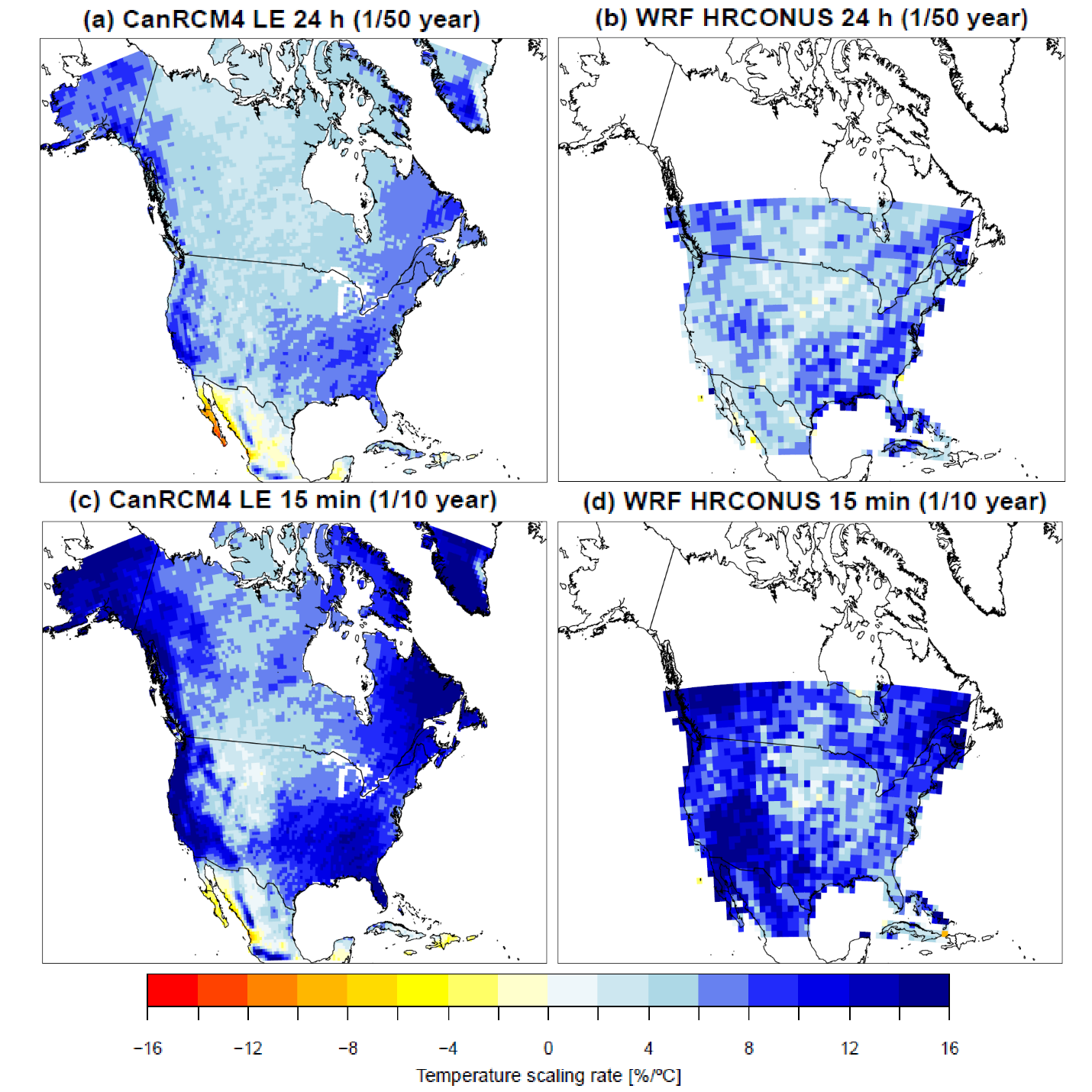
The broad consistency of results at a regional scale suggest that it might be possible to very cautiously apply results from CanRCM4 despite the fact that it does not represent convection explicitly. This is supported by comparisons between observed NBCC 2015 Table C-2 15-min rainfall design data and those extrapolated from CanRCM4 LE to the 15-min duration based on temporal simple scaling (Figure 4.6). There is an acceptable degree of correspondence in the historical period (1986-2016) both in terms of pattern (explained variance r2 = 0.7) and magnitude (interquartile range of relative errors of -6% to +19%).
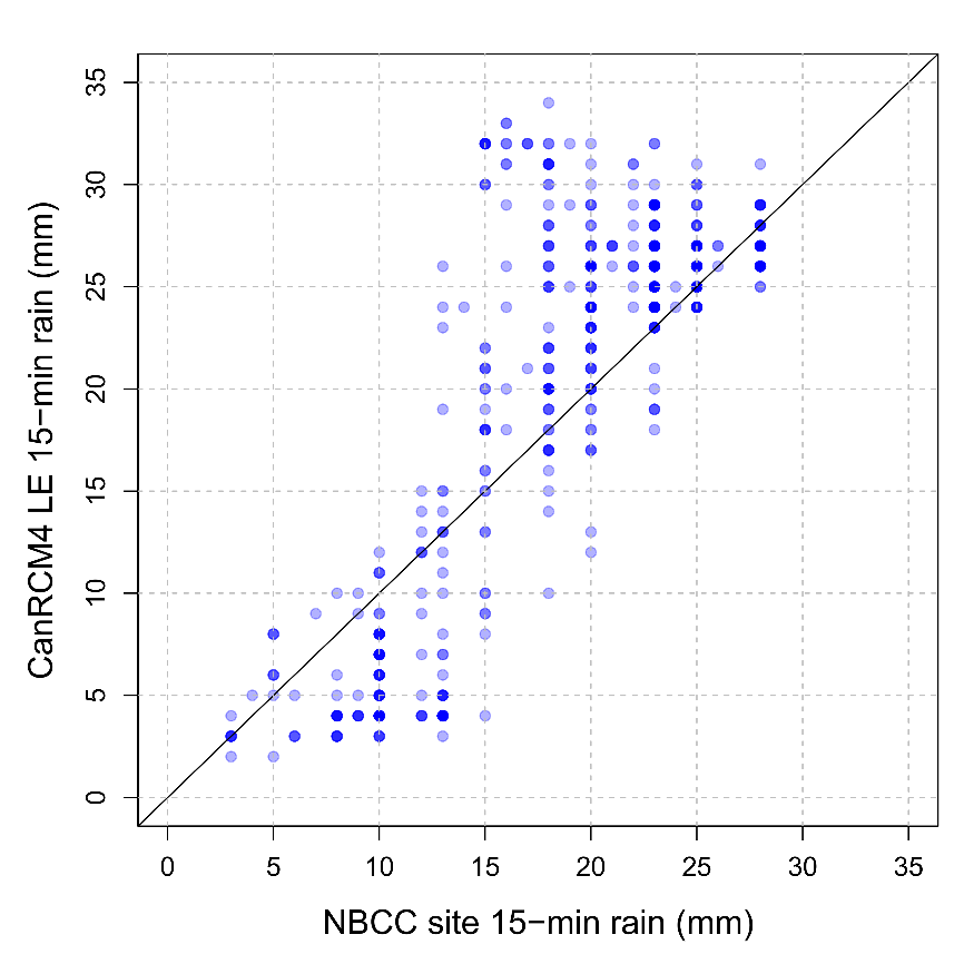
4.2.3 Interpretation
One day (50-year return period) and 15-min (10-year return period) rain are Tier 2 variables. The CCCR (Bush and Lemmen, 2019)Reference 3 finds that it is likely that extreme precipitation will increase in Canada in the future, although the magnitude of the increase at regional scales is much more uncertain.
Given that more confidence can be placed on regional temperature projections, the use of temperature scaling factors – expressing the relative change in precipitation extremes as a function of warming – is recommended. This is consistent with other national recommendations (e.g., Ball et al., 2016; Book 1, Ch. 6)Reference 55 and is also motivated by the fact that atmospheric moisture is expected to scale approximately exponentially with warming at a rate of ~7%/°C according to the CC relationship. A reasonable expectation would be for the intensity of rare precipitation extremes to follow suit to first order if thermodynamic influences dominate over dynamical changes.
Based on targeted research involving simulations from CanRCM4 LE and convection-permitting simulations from WRF HRCONUS, it is found that extreme precipitation scales roughly with local annual mean temperature at rates similar to that predicted by the CC relation. Nevertheless, exact values are hard to estimate for several reasons: (1) long record lengths are needed to constrain the estimation (Li et al., 2019a)Reference 36; (2) scaling factors appear to be larger in some regions, especially along the coasts, than in other regions, in particular in the interior of Canada to the east of the Rockies (Li et al., 2019aReference 36; Cannon and Innocenti, 2019Reference 64); and (3) scaling rates tend to be larger for shorter durations and for rarer, more extreme events (Li et al., 2019aReference 36; Cannon and Innocenti, 2019Reference 64). Results from CanRCM4 LE and WRF HRCONUS are broadly consistent (Figure 4.4 and Figure 4.5).
This research suggests that there may be a need for detailed scaling rates that are specific to different regions, different types/level of extremes, including daily, sub-daily, and sub-hourly events, and different event rarities. There are, however, problems in doing so, since estimates become less robust at this level of detail, due to (1) assumptions involved in the statistical analyses; (2) the modest resolution of conventional RCMs; (3) the limited number of RCMs with simulations of sufficient length; (4) the very limited number of continental-scale convection-permitting simulations; and (5) the low signal-to-noise ratio of forced changes in precipitation extremes relative to internal variability (values of NS ratio for direct estimates of one day 50-year return period rain are >0.8 at all global warming levels). Thus, confidence in estimates of any specific scaling rate corresponding to different events in different regions is very low to low. On balance, it is therefore not possible to provide detailed projections based on existing model simulations.
For these reasons, at this time it is recommended that scaling of extreme one day (50-year return period) and 15-min (10-year return period) rain design data follow the CC relation of 7%/°C of local warming based on local annual mean temperature change (see chapter 2) and hence the place-specific projections provided in Appendix 1.2 are based on CanRCM4 LE temperature projections. Confidence in these place specific projections is limited, not only because confidence is necessarily lower at finer spatial and temporal scales, but also because of their indirect nature. More than one line of evidence suggests that extreme precipitation scales with temperature in most Canadian land regions in a way that is roughly consistent with the theoretical CC relationship. There is, however, also evidence of deviations from this rate regionally (with lower than CC rates in continental climate areas to the east of the Rockies), for different accumulation durations (higher for shorter durations), and different event rarities (higher for more rare events), albeit with very low to low confidence on such details.
4.3 Annual relative humidity
4.3.1 Assessment
The moisture index in the NBCC relies, in part, on relative humidity, and the CHBDC includes a map of historical annual relative humidity. The distribution of tropospheric moisture is strongly constrained by the fact that moisture condenses out of supersaturated air. As almost all air parcels will reach saturation during their lifetimes, it is thus plausible that the distribution of relative humidity will remain roughly unchanged under climate change. For high latitudes, where air is usually closer to saturation, this constraint is strong and is reflected by the fact that relative humidity is roughly constant through the substantial temperature changes of the seasonal cycle. According to IPCC (2007)Reference 72, “a broad-scale, quasi-unchanged [relative humidity] response [to climate change] is uncontroversial”.
More recent analyses of projections from CMIP3 and CMIP5 GCMs reveal additional details, including a small near-surface drying signal over most global land areas, albeit with large uncertainty. For CMIP3 GCMs, O’Gorman and Muller (2010)Reference 73 found a modest sensitivity of surface relative humidity to global warming, with ensemble mean values changing at a rate of between approximately -0.7% and +0.7% per °C over Canadian land regions. CMIP5 GCMs (IPCC, 2013)Reference 4 project a decrease of between 0% and approximately 2% in annual mean relative humidity over Canada (2081-2100 RCP8.5 with respect to 1986-2005). This change, however, is not considered to be a robust feature of the CMIP5 projections (Collins et al., 2013, Figure 12.21)Reference 74.
4.3.2 Targeted research
As described in chapter 1, the approach recommended for B&CPI is to communicate regional changes in annual relative humidity that are tied to fixed levels of global warming. Projections of annual mean relative humidity by CanRCM4 LE show little to no change over Canada (Figure 4.7). Scaling of regional changes in relative humidity with global warming is summarized in Figure 4.8 and Table 4.2. While increases in relative humidity are projected over all regions, the magnitude of change is small (no greater than +0.65%/°C global warming). Confidence in this change, which deviates from CMIP5 results assessed in IPCC (2013)Reference 4, is very low.
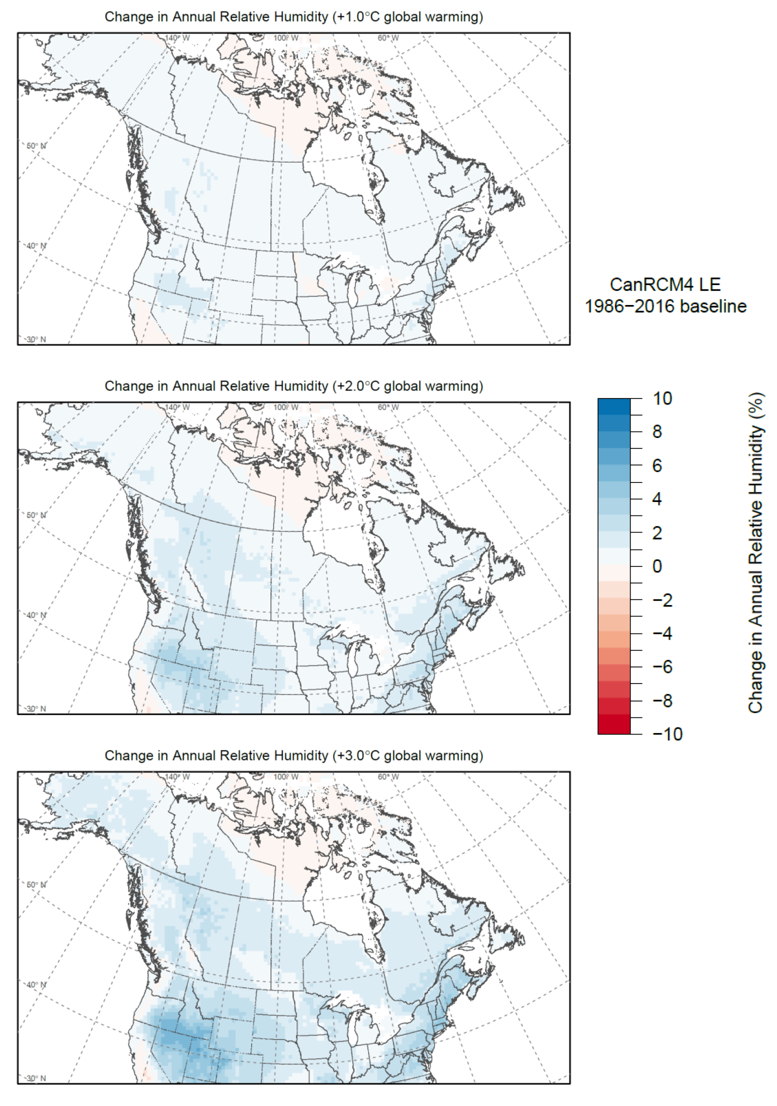
Table 4.2: Projected changes in annual relative humidity for locations approximating Table C-2 locations in six Canadian regions and Canada as a whole for +1°C, +2°C, and +3°C global warming levels with respect to the 1986-2016 baseline period. Values represent the ensemble projection (25th percentile, 75th percentile) calculated from CanRCM4 LE.
| Change in ann. rel. hum. [%] | Global warming level | ||
|---|---|---|---|
| Region | +1°C | +2°C | +3°C |
| British Columbia | 0.4 (0.2, 0.7) | 0.6 (0.4, 0.9) | 0.7 (0.5, 1.0) |
| Prairies | 0.5 (0.0, 1.0) | 1.0 (0.4, 1.5) | 1.3 (0.8, 1.9) |
| Ontario | 0.1 (-0.1, 0.3) | 0.3 (0.0, 0.6) | 0.7 (0.5, 0.9) |
| Quebec | 0.5 (0.3, 0.7) | 1.1 (0.8, 1.3) | 1.9 (1.6, 2.1) |
| Atlantic | 0.5 (0.4, 0.7) | 1.1 (1.0, 1.2) | 1.7 (1.6, 1.9) |
| North | 0.3 (0.1, 0.4) | 0.5 (0.3, 0.6) | 0.8 (0.6, 0.9) |
| Canada | 0.3 (0.1, 0.6) | 0.8 (0.5, 1.1) | 1.3 (0.9, 1.6) |
4.3.3 Interpretation
Annual mean relative humidity is a Tier 3 variable. On very large spatial scales, IPCC (2007)Reference 72 states that “a broad-scale, quasi-unchanged [relative humidity] response [to climate change] is uncontroversial”. There is generally high confidence that future changes in relative humidity will be small. IPCC (2013)Reference 4 finds that “although the CMIP5 projected changes are small [there is] medium confidence that reductions in near-surface [relative humidity] over many land areas are likely.” In contrast, CanESM2-CanRCM4 LE suggests a small increase in relative humidity, with increases of less than about +0.65%/°C global warming in all regions.
Projected changes in annual relative humidity at locations approximating Table C-2 locations are provided in Appendix 1.2. As was the case for annual mean temperature, values are derived directly from CanRCM4 LE projections for each global warming level. Because the climate change signal is so small at low levels of global warming, values of NS ratio are typically quite high – the magnitude of regional change and internal variability are of the same order up to approximately +1.5°C global warming. These estimates of what is a very small signal could perhaps be useful in cases where the objective is to ensure conservative designs that minimize the risk of future load exceedance, for example, when determining the required capacity of a cooling plant for a large building.
5. Wind pressures
5.1 Hourly wind pressures
5.1.1 Assessment
Wind loads are specified to consider external pressures or suctions caused by strong winds on the main structural systems and all secondary components of buildings or structures. Wind loads are also used to design flexible structures, such as tall buildings and bridges, which require consideration of wind-induced oscillations and vibrations. In the NBCC, design wind pressures for 10 and 50-year return periods are determined based on the design wind speeds for the same return periods estimated from the Gumbel distribution fitted to observed annual maxima of hourly wind speeds recorded at a standard anemometer height of 10 m above the ground. The CHBDC further includes 25 and 100-year return periods. Wind pressure is directly proportional to the square of the wind speed.
Historical and projected changes in wind speed over Canada were not assessed as part of the CCCR (Bush and Lemmen, 2019)Reference 3. Relative to the body of literature for variables such as temperature and precipitation, much less attention has been paid to wind extremes and hence, overall uncertainty about historical trends and future changes is also higher. Some studies (e.g., Vautard et al., 2010Reference 75; McVicar et al., 2012Reference 76) have assessed historical trends in surface (10 m) mean and extreme wind speeds and reported general decreasing trends in observations across the globe. In particular, decreases in surface mean wind speeds by 5-15% were noted by Vautard et al. (2010)Reference 75 in observations from meteorological stations in all continental areas in the northern midlatitudes for the 1979-2008 period. It is, however, unclear to what extent decreasing trends are due to climatic factors or non-climatic factors that affect observations (e.g., changes in surface roughness in the vicinity of the anemometer, anemometer height, and other measurement practices). Also, the relationships between trends in mean wind speeds and those in extreme winds are still not well understood (IPCC, 2012)Reference 77.
Over Canada, surface wind speeds exhibit both decreasing and increasing trends depending on regions or seasons. Wan et al. (2010)Reference 78 reported decreases in hourly surface wind speed for western Canada and most parts of southern Canada for all four seasons, but increases in the central Canadian Arctic for all seasons and for the Maritimes during spring and autumn. Li et al. (2017)Reference 79 analyzed trends in observed annual maximum wind speed at stations in major cities across Canada. They found that 6 of 20 stations exhibited significant decreasing trends, which is supportive of a general decline.
Several studies have evaluated projected changes to mean and extreme wind speeds over North America using multi-model ensembles of GCMs. For instance, Mclnnes et al. (2011)Reference 80 showed increases in mean wind speeds for southeastern and northern parts of North America at the end of this century based on the CMIP3 multi-model ensemble under the IPCC SRES (2000) A1B emissions scenarioReference 145. Kumar et al. (2015)Reference 81 considered changes in wind extremes at the end of this century based on the CMIP5 multi-model ensemble under the RCP8.5 scenario and found modest changes of mixed sign over Canada representing changes in magnitude of no more than a few percent. IPCC (2012)Reference 77, however, highlighted that there is low confidence in the projected changes to extreme winds obtained from GCMs because relatively few studies have assessed extreme winds and because GCMs cannot resolve all of the mechanisms that produce extreme wind events, such as small-scale storms. To the extent that CMIP5 GCMs do project changes in surface winds, it is unclear whether these arise due to circulation change or other causes, such as changes in surface roughness due to changes in surface vegetation simulated by the terrestrial ecosystem components of these models.
Recent assessments of observed and projected changes in tropical cyclone activity (Knutson et al., 2019, 2020)Reference 82Reference 83 suggest that global average tropical cyclone intensity and the proportion of tropical cyclones that reach very intense levels will increase with global warming (medium to high confidence), including attendant increases in wind speed, but that this may be accompanied by either unchanged or reduced frequency of tropical cyclones over all categories (medium confidence). The net effect on the frequency of intense tropical cyclones is thus uncertain. There is medium confidence that there will be a poleward expansion of the position of maximum tropical cyclone intensity in the western North Pacific and that tropical cyclone translation speeds will slow.
The ability to represent extratropical cyclones in GCMs has been improving, partly due to increases in horizontal resolution, although most models still underestimate extratropical cyclone frequency and intensity (Colle et al., 2013Reference 84; Zappa et al., 2013Reference 85). Dynamical downscaling with an RCM can help to reduce biases in extratropical cyclone frequency and intensity, but does not eliminate those biases, as Seiler, et al. (2018)Reference 32 show in a study using CanESM2 and CanRCM4. More generally, the dynamical response to global warming is felt to be uncertain and modest (Deser et al., 2012Reference 15; Shepherd, 2014Reference 86; Trenberth, 2015Reference 87). This is supported indirectly by the absence of detection and attribution results concerning storm frequency, intensity or location and lack of a robust literature on the detection and attribution of changes in the global surface pressure distribution.
RCMs also have been employed in regional-scale studies to analyze climate change impacts on mean and extreme wind speeds. Over the US, Pryor et al. (2012)Reference 88 evaluated future wind climates based on an ensemble obtained from North American Regional Climate Assessment Program (NARCCAP) under the IPCC SRES A2 emissions scenario for the middle of the current century (2041-2062). They found some decreases in mean wind speeds over the western US, but no significant differences in extreme wind speeds in the future. A study of regional-scale projections of extreme wind speeds over Canada and associated changes in design wind pressures for buildings and structures was conducted by Jeong and Sushama (2018a)Reference 89 using the CRCM5 regional climate model with 0.44° grid spacing. They considered CRCM5 simulations driven by simulations from two GCMs under the RCP4.5 and RCP8.5 emissions scenarios. While some scattered increases in the magnitude of future 50-year return period wind speeds and pressures were found, the changes were not found to be statistically robust, with individual simulations showing dissimilar patterns of projected change, indicating that differences were likely due to internal variability rather than external forcing.
A more robust assessment of climate change signals in design wind loads may ultimately be obtained from wider study of RCMs with much higher resolution than used in most current research today. In an early study, Pryor et al. (2012)Reference 88 showed that an increase in RCM resolution from 50 km to 6 km increased extreme wind speeds more than the mean wind speed. More recently, Prein et al. (2017a)Reference 90 reported changes in the characteristics of mesoscale convective systems, which often produce high winds, in the WRF HRCONUS convection-permitting model simulations over North America (see also section 4.2.2). Results from such models are dependent on modelling strategy and remain limited in geographical extent and simulation length due to their very high computational cost.
Studies of extreme wind speed projections in North America show some agreement that future changes will be small. However, there is generally low confidence in projected changes to extreme winds because GCMs cannot resolve many of the mechanisms that produce extreme wind events and RCMs also have biases in frequency and intensity of low-pressure systems. Based on the limited scientific literature, low signal-to-noise ratio in the projected changes to extreme winds, and the general inability of conventional RCMs to simulate extreme winds associated with small scale processes such as mesoscale convective systems, there is very low confidence in projections of future design wind pressures in Canada.
5.1.2 Targeted research
Given the paucity of research and climate model simulations related to sub-daily wind speed extremes in Canada, the literature assessment in this project is supplemented by an analysis of projected changes to design wind pressures, and their internal variability, from the CanESM2-CanRCM4 LE. The reference hourly wind speed observations from which NBCC design wind loads were derived include wind records from about 135 stations with hourly mean wind speeds and from 465 stations with aviation (one- or two-minute average) wind speeds or surface weather (ten-minute average) wind speeds observed once per hour at the top of the hour (NRC, 2015)Reference 1. The CanRCM4 simulations are run with a time step of 20-min, and thus the wind speed that is simulated in a given time step for a particular grid box should be considered as the speed of the average wind in the grid box during the 20-minute period. Note however that variations from one time step to the next are unlikely to be realistic since such variations occur at timescales shorter than the model’s “skillful scale” (see section 4.2.2). Nevertheless, an extreme value analysis is performed on the annual maxima of the daily maximum 10 m wind speed variable from CanRCM4 – the maximum wind speed of all time steps from 00:00 UTC to 00:00 UTC the next day – at each grid cell using the extreme value analysis approach adopted in the NBCC. In particular, the Gumbel distribution is fitted via the method of moments to 20-min wind speed annual maxima using the 31-year period associated with each level of global warming. Wind speeds for the design return periods are estimated first, and then wind pressures are calculated following NRC (2015)Reference 1. This is done for each of the 50 ensemble members separately to estimate ensemble spread due to internal variability. Wind speeds are converted to wind pressures, and projected changes to the magnitude of design pressures for 10, 25, 50, and 100-year return periods were estimated at specific levels of future global mean temperature change (e.g., +1, +2, and +3°C) above the 1986-2016 baseline level.
A dynamic vegetation model was used for calculations involving the land carbon cycle in the global CanESM2 simulations that drive CanRCM4. In CanESM2, crop area increases over the historical period and then changes in response to the climate in the future. Vegetation also grows and dies in response to changes in climate, and so vegetation height and thus surface roughness length are nonstationary. This produces discernable changes in 10 m winds in CanESM2, but it seems unlikely that the nonstationary surface roughness length in CanESM2 would have discernably affected CanRCM4 since CanESM2 surface winds are not used to drive CanRCM4. Only CanESM2 atmospheric model level winds are used for that purpose. The variations in surface roughness would only have very weakly affected CanESM2 winds on atmospheric model levels within the planetary boundary layer and would likely have had no effect above the planetary boundary layerFootnote 10x. Also, the dynamic vegetation scheme was switched off and thus surface roughness length does not change over time within CanRCM4. For these two reasons, it is safe to conclude that any changes in surface wind speed in CanRCM4 are not caused by changes in surface roughness.
CanRCM4 LE projects increases (mostly less than 10% for the +3°C global warming level) to the 50-year return period design wind pressures over Canada (Figure 5.1). Higher inter-annual variability, as shown by increases in the coefficient of variation (CoV), the ratio of the standard deviation of annual maximum wind speed to the mean of annual maximum wind speed, is a main contributor to projected increases in the design wind pressure at different global warming levels (Table 5.1 and Table S5.1). British Columbia, Ontario, and Atlantic regions show larger increases in the design wind pressures compared to the other regions, and the relative magnitude of the increases scale roughly linearly with global warming level (Figure 5.2). For reference, projected changes in the 10-year return period design wind pressure are provided in Figure 5.3, Figure 5.4 and Table 5.2; they show similar behavior to those of the 50-year return period. The spatial patterns of the projected changes to extreme wind speeds and pressures from CanRCM4 LE are generally consistent with findings from GCMs (McInnes et al., 2011Reference 80; Kumar et al., 2015Reference 81) and other RCMs (Jeong and Sushama, 2018a)Reference 89. Projected changes in the mean and CoV of annual maximum wind speed are provided as supplemental material in Table S5.1.
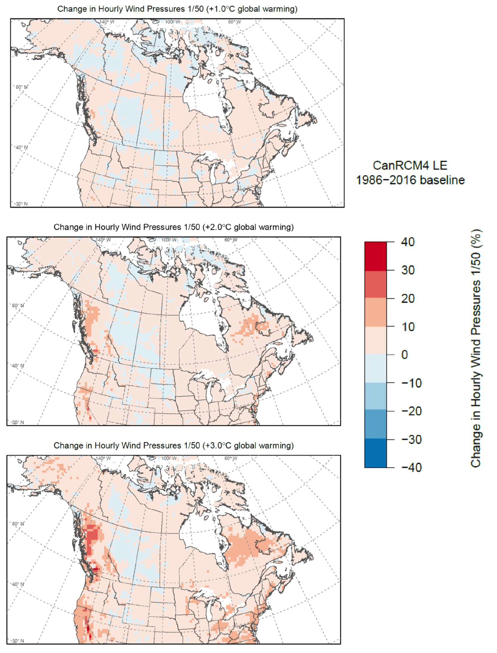
Table 5.1: Projected changes to 50-year return period hourly wind pressure (upper panel) and coefficient of variation (CoV) of annual maximum hourly wind pressure (bottom panel) for locations approximating Table C-2 locations in six Canadian regions and Canada as a whole for +1°C, +2°C, and +3°C global warming levels with respect to the 1986-2016 baseline period. Values represent the ensemble projection (25th percentile, 75th percentile) calculated from CanRCM4 LE.
| Change in hourly wind pressures 1/50 [%] | Global warming level | ||
|---|---|---|---|
| Region | +1°C | +2°C | +3°C |
| British Columbia | 1.1 (-5.7, 7.8) | 3.9 (-3.2, 13.5) | 7.4 (-0.2, 19.1) |
| Prairies | -0.6 (-6.7, 6.0) | -0.2 (-7.1, 7.0) | 0.0 (-6.7, 7.2) |
| Ontario | 2.1 (-5.5, 10.6) | 4.8 (-3.9, 14.4) | 8.5 (-0.8, 18.6) |
| Quebec | 1.6 (-5.2, 9.0) | 2.6 (-4.9, 11.8) | 4.1 (-4.3, 12.2) |
| Atlantic | 2.9 (-4.5, 11.0) | 5.8 (-3.8, 15.1) | 6.2 (-2.2, 15.8) |
| North | -0.6 (-7.3, 6.9) | 0.6 (-7.2, 9.2) | 1.6 (-6.1, 10.4) |
| Canada | 1.6 (-5.6, 9.3) | 3.6 (-4.7, 12.3) | 5.3 (-3.2, 14.4) |
| Change in hourly wind pressures CoV [%] | Global warming level | ||
|---|---|---|---|
| Region | +1°C | +2°C | +3°C |
| British Columbia | 0.6 (-11.1, 13.8) | 2.3 (-10.8, 16.5) | 6.5 (-6.8, 24.6) |
| Prairies | 1.4 (-10.4, 15.4) | 4.2 (-9.8, 20.1) | 7.6 (-6.3, 23.6) |
| Ontario | 2.3 (-10.4, 18.1) | 5.3 (-9.1, 23.2) | 10.2 (-4.9, 27.1) |
| Quebec | 0.0 (-10.6, 12.9) | 0.7 (-12.1, 17.3) | 1.5 (-12.5, 17.0) |
| Atlantic | 1.6 (-12.0, 16.8) | 3.0 (-11.4, 20.4) | 3.1 (-10.0, 20.0) |
| North | -1.6 (-12.6, 11.2) | 0.3 (-13.3, 15.3) | 1.4 (-13.2, 15.4) |
| Canada | 1.3 (-10.9, 15.1) | 3.0 (-10.5, 19.6) | 5.1 (-9.2, 21.0) |
Table S5.1: Projected changes to the mean and coefficient of variation (CoV) of annual maximum hourly wind speed for locations approximating Table C-2 locations in six Canadian regions and Canada as a whole for global warming levels from +0.5°C to +3.5°C with respect to the 1986-2016 baseline period. Values represent the ensemble projection (25th percentile, 75th percentile) calculated from CanRCM4 LE.
| Change in hourly wind speed mean [%] | Global warming level | ||||||
|---|---|---|---|---|---|---|---|
| Region | +0.5°C | +1°C | +1.5°C | +2°C | +2.5°C | +3°C | +3.5°C |
| British Columbia | 0.1 (-1.0, 1.4) | 0.2 (-1.3, 1.8) | 0.9 (-0.8, 2.7) | 1.8 (0.2, 3.4) | 2.1 (0.1, 4.1) | 2.3 (0.5, 4.7) | 2.1 (0.2, 4.1) |
| Prairies | -0.3 (-1.3, 0.7) | -0.6 (-1.9, 0.9) | -0.8 (-2.2, 0.6) | -1.1 (-2.6, 0.6) | -1.2 (-2.7, 0.4) | -1.6 (-3.0, 0.0) | -1.9 (-3.4, -0.3) |
| Ontario | 0.4 (-0.6, 1.6) | 0.6 (-1.0, 2.2) | 0.8 (-1.1, 2.7) | 1.1 (-0.8, 2.9) | 1.6 (-0.1, 3.3) | 1.9 (-0.1, 4.0) | 2.1 (0.1, 4.1) |
| Quebec | 0.5 (-0.7, 1.5) | 0.7 (-0.8, 2.3) | 0.9 (-0.7, 2.5) | 1.3 (-0.6, 3.1) | 1.4 (-0.5, 3.3) | 1.4 (-0.5, 3.4) | 1.4 (-0.4, 3.4) |
| Atlantic | 0.7 (-0.6, 2.0) | 1.1 (-0.6, 3.0) | 1.6 (-0.3, 3.3) | 2.0 (0.2, 3.9) | 2.4 (0.3, 4.2) | 2.4 (0.4, 4.4) | 2.8 (0.8, 4.7) |
| North | 0.0 (-1.2, 1.3) | 0.0 (-1.7, 1.6) | 0.1 (-1.7, 2.0) | 0.5 (-1.5, 2.3) | 0.9 (-1.1, 2.7) | 1.0 (-1.0, 3.0) | 1.2 (-0.6, 3.0) |
| Canada | 0.4 (-0.8, 1.4) | 0.5 (-1.1, 2.1) | 0.8 (-1.0, 2.4) | 1.0 (-0.7, 2.8) | 1.4 (-0.4, 3.3) | 1.5 (-0.3, 3.5) | 1.6 (-0.1, 3.5) |
| Change in Hourly Wind Speed CoV [%] | Global warming level | ||||||
|---|---|---|---|---|---|---|---|
| Region | +0.5°C | +1°C | +1.5°C | +2°C | +2.5°C | +3°C | +3.5°C |
| British Columbia | 0.2 (-8.8, 8.8) | 0.6 (-11.1, 13.8) | 1.6 (-11.5, 16.3) | 2.3 (-10.8, 16.5) | 5.5 (-8.2, 23.5) | 6.5 (-6.8, 24.6) | 7.9 (-6.2, 25.9) |
| Prairies | 1.8 (-6.8, 10.1) | 1.4 (-10.4, 15.4) | 2.7 (-10.8, 18.1) | 4.2 (-9.8, 20.1) | 7.0 (-6.8, 23.0) | 7.6 (-6.3, 23.6) | 9.9 (-4.3, 25.1) |
| Ontario | 0.9 (-8.1, 12.2) | 2.3 (-10.4, 18.1) | 3.5 (-10.9, 19.8) | 5.3 (-9.1, 23.2) | 8.4 (-5.9, 26.8) | 10.2 (-4.9, 27.1) | 13.2 (-3.0, 31.2) |
| Quebec | -1.5 (-10.8, 8.6) | 0.0 (-10.6, 12.9) | 0.7 (-10.1, 15.2) | 0.7 (-12.1, 17.3) | 0.2 (-13.5, 15.4) | 1.5 (-12.5, 17.0) | 1.1 (-11.6, 17.6) |
| Atlantic | 0.2 (-10.1, 9.8) | 1.6 (-12.0, 16.8) | 2.5 (-12.4, 19.0) | 3.0 (-11.4, 20.4) | 2.9 (-11.8, 18.2) | 3.1 (-10.0, 20.0) | 4.7 (-8.0, 21.8) |
| North | -0.2 (-8.3, 9.4) | -1.6 (-12.6, 11.2) | -1.2 (-13.3, 12.4) | 0.3 (-13.3, 15.3) | 0.6 (-12.2, 16.5) | 1.4 (-13.2, 15.4) | 1.6 (-12.1, 17.0) |
| Canada | 0.3 (-8.7, 9.9) | 1.3 (-10.9, 15.1) | 1.8 (-11.0, 17.3) | 3.0 (-10.5, 19.6) | 4.1 (-9.2, 20.8) | 5.1 (-9.2, 21.0) | 6.2 (-7.5, 23.6) |
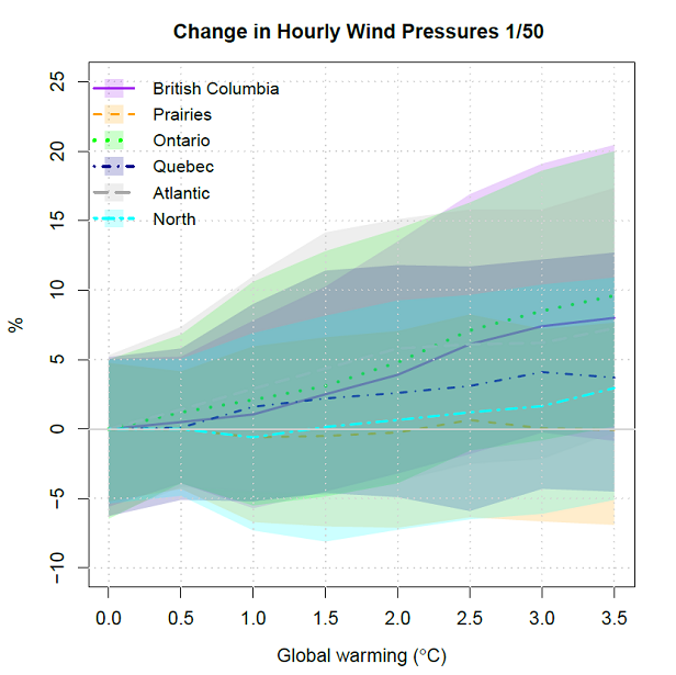
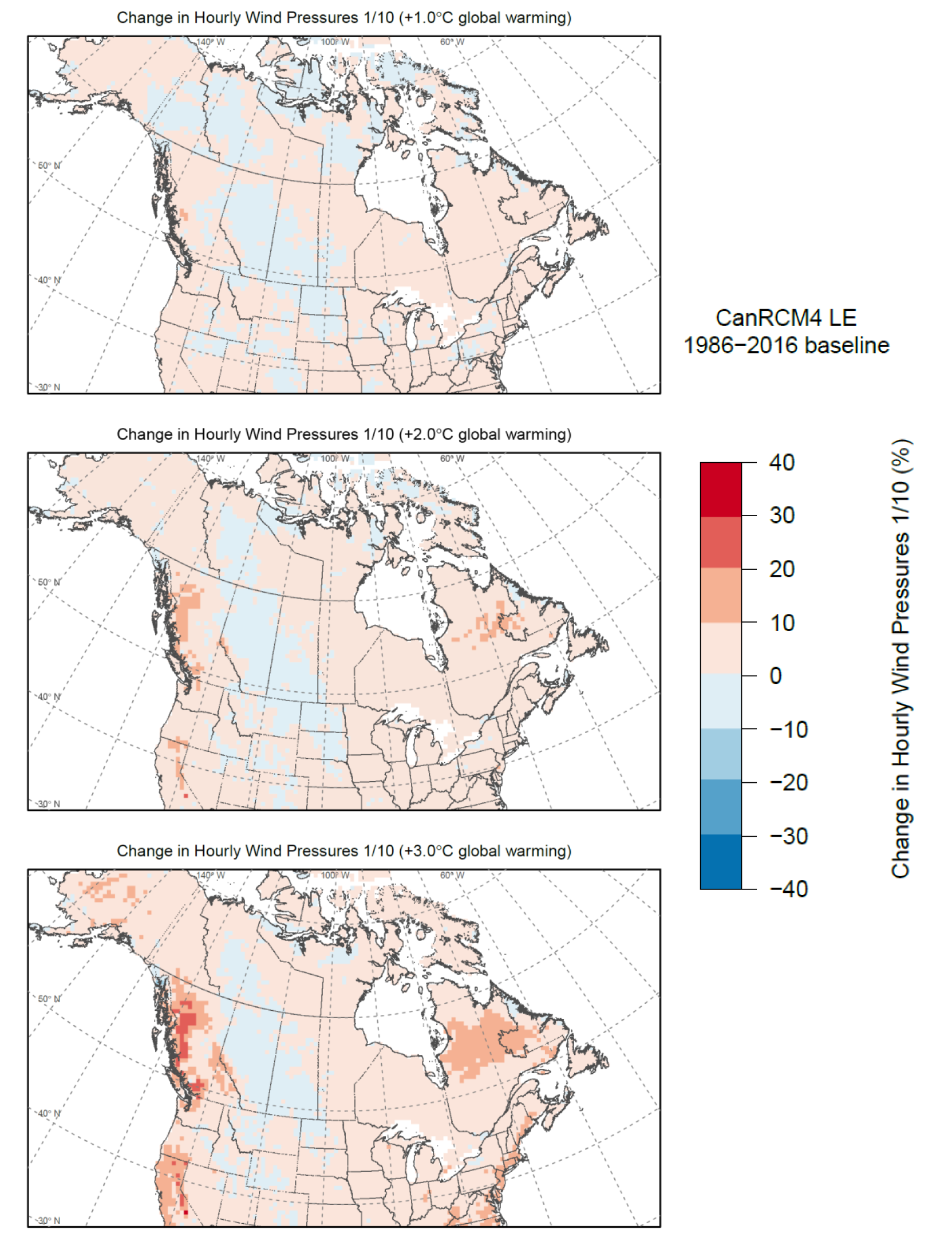
Table 5.2: Projected changes (in percent) to 10-year return period hourly wind pressures for locations approximating Table C-2 locataions in six Canadian regions and Canada as a whole for +1°C, +2°C, and +3°C global warming levels with respect to the 1986-2016 baseline period. Values represent the ensemble projection (25th percentile, 75th percentile) calculated from CanRCM4 LE.
| Change in hourly wind pressures 1/10 [%] | Global warming level | ||
|---|---|---|---|
| Region | +1°C | +2°C | +3°C |
| British Columbia | 0.7 (-3.9, 5.5) | 3.7 (-1.4, 9.7) | 6.2 (-0.9, 14.1) |
| Prairies | -0.9 (-5.2, 3.9) | -1.1 (-5.8, 3.9) | -1.4 (-6.0, 3.7) |
| Ontario | 1.8 (-3.6, 7.7) | 3.6 (-2.3, 10.3) | 6.7 (0.0, 13.6) |
| Quebec | 1.3 (-2.9, 6.9) | 2.6 (-3.0, 8.9) | 3.5 (-1.9, 9.3) |
| Atlantic | 2.5 (-3.0, 8.2) | 4.8 (-1.2, 11.6) | 5.1 (-0.9, 12.4) |
| North | -0.3 (-5.3, 5.2) | 0.6 (-4.8, 6.5) | 1.7 (-3.5, 7.5) |
| Canada | 1.3 (-3.8, 6.9) | 3.1 (-3.0, 9.4) | 4.4 (-1.5, 10.6) |
Confidence in these projections is very low. Projected changes are subject to large internal variability; the ensemble spread in projections from CanRCM4 LE is large relative to the magnitude of the forced change for all Canadian regions (Table 5.1 and Table 5.2; Figure 5.2 and Figure 5.4), indicating high uncertainty just from natural variability of the climate system and suggesting that no change is a plausible outcome for all regions. There is also large uncertainty related to the models themselves that is much more difficult to quantify. Circulation changes in the GCMs are weak and inconsistent, biases in the simulation of large-scale low pressure systems that remain after dynamical downscaling (e.g., Seiler et al., 2018)Reference 32 and GCMs and RCMs have insufficient resolution to represent small-scale phenomena such as tornados and convective wind storms.
5.1.3 Interpretation
Design wind pressure is a Tier 3 variable that has very low confidence in the future projection. Projected changes at locations approximating Table C-2 locations are provided in Appendix 1.2; results from CanRCM4 LE are cautiously provided for each global warming level for illustration purposes, with the strong caveat that little confidence can be placed in the projections at this time. They should only be used to explore possible future load scenarios, bearing in mind that changes could very well be underestimated given the limitations of the modelling systems on which they are based. In general, CanRCM4 LE projects small changes in the future design wind pressures (generally less than +/-10% at +3°C global warming level relative to the baseline) with high internal variability and uncertainty. Values of NS ratio for wind loads tend to be close to one at all global warming levels. While there is some consistency amongst projections by different models that changes in future design wind pressures over Canada will be small (e.g., Kumar et al., 2015Reference 81; Jeong and Sushama, 2018aReference 89), this is subject to very high uncertainty due to lack of consensus amongst models on global patterns of the dynamical response to external forcing, the low signal-to-noise ratio and the general inability of conventional RCMs to adequately represent many of the physical processes that drive extreme winds.
5.2 Driving rain wind pressures
5.2.1 Assessment
Driving rain wind pressures (DRWPs) are considered in the design and construction of buildings because high wind pressure in the presence of rainwater can result in damage to building envelopes by promoting inflow of water through joints, cracks, or porous exterior surfaces. In the NBCC, DRWP is defined as the hourly wind pressure with rainfall exceeding a certain threshold (i.e., 1.8 mm/hr). The design DRWP for the 5-year return period is estimated from the Gumbel distribution fitted to the annual maximum series of hourly DRWPs.
Most studies have focused on the estimation of historical values of DRWP using meteorological observations over different parts of the world, including Japan (Murakami et al., 1987)Reference 91, Australia (Choi, 1992)Reference 92, Chile (Pérez-Bella et al., 2013)Reference 93, Spain (Pérez-Bella et al., 2014)Reference 94, and Canada (Welsh et al., 1989Reference 95; Cornick and Lacasse, 2005Reference 96). In Canada, Welsh et al. (1989)Reference 95 constructed a map and table for 5-year return period DRWP, which have been used in the design of residential and commercial buildings as well as their door and window systems (CSA, 2018)Reference 97.
As discussed in section 5.1 above, the limited number of observational studies tend to find weakening surface winds globally, and an equivocal set of findings in Canada, with regional variations in the direction of trend. Several modelling studies have evaluated projected changes in mean or extreme wind speeds for by the end of this century, based on the CMIP3 and CMIP5 multi-model ensemble projections. These indicate only modest changes over Canada, with little consensus on the direction of change. The magnitude of change could be underestimated given model limitations. Overall, there is very low confidence in the projections due to low signal-to-internal-noise ratios and high levels of model uncertainty.
As discussed in chapter 4, the CCCR found observational evidence for increases in annual total precipitation over Canada, with proportionally larger increases in winter and in northern Canada (Bush and Lemmen, 2019)Reference 3. Confidence in direct model projections of changes in precipitation frequency and intensity is limited by modelling uncertainty and relatively low signal-to-internal noise ratios. Temperature, however, is an important consideration when considering DRWP since this affects the relative frequency of rainfall events. Canada is projected to warm more than the global mean, with even larger increases in winter and in northern Canada. Increases in surface air temperature will lead to a shift in precipitation type from snow to rain, which, in turn, will result in increases in the frequency of rainfall from autumn to spring over Canada (Harder et al., 2015Reference 98; Jeong and Sushama, 2018bReference 31).
Therefore, it is plausible that changes in rainfall occurrence and amount in a future warmer climate could have some implications for design DRWPs even if there is little overall change in wind speeds. Note that these changes could occur in at least three ways – either because winds do strengthen, an aspect with very low confidence, or because the number of driving rain events increases, increasing the size of the annual sample of hourly wind speeds from which the annual maximum is extracted, or because the annual period during which DRWP events can occur extends into climatologically windier parts of the year, an aspect in which there might be higher confidence. Unfortunately, few studies have quantified future changes in the combined occurrence of wind and rain and their impacts on buildings. One exception is Nik et al. (2015)Reference 99 who investigated future moisture loads for building façades caused by wind-driven rain in Sweden using Swedish RCM simulations, and found that higher amounts of moisture accumulate in building walls in the future. Nevertheless, studies to evaluate projected changes to DRWPs are not yet available for many countries, including Canada.
While few studies have considered projected changes in DRWP and there is very low confidence in projections of future design wind pressures in Canada, greater understanding of projected increases in temperature and precipitation, and hence rainfall, leads to medium confidence that future design DRWP will increase in Canada.
5.2.2 Targeted research
Given that very few studies have considered projected changes to compound wind and rain extremes, the literature assessment in this project is supplemented by an analysis of projected changes to DRWP based on hourly outputs from the CanESM2-CanRCM4 LE. For gauge observations, DRWP is calculated from time series of annual maximum 1-hour wind speeds that coincide with rainfall in excess of 1.8 mm/hr. The same 1.8 mm/hr threshold is applied in calculations based on CanRCM4 LE outputs, which means that rainfall rates are analyzed at the grid cell scale in the model and at the point scale in observations.
The extreme value analysis for the combined wind and rain hazard simulated by CanRCM4 differs slightly from that used for design wind pressures. The additional requirement that extreme wind speeds occur at the same time as rainfall reduces the number of CanRCM4 LE members from 50 to 15, as only 15 members archived the high-frequency variables needed to calculate both 1-hour wind speed and 1-hour rainfall. In both cases, wind and rain variables are mean values taken over three 20-minute time steps. This differs from the daily maximum 20-min time step wind variable used to compute design wind pressures.
Future projections of DRWP are partly dependent on the ability of CanRCM4 to correctly simulate the frequency of hourly rainfalls in excess of the threshold; hence, climate model biases – in this case systematic differences between the simulated historical and observed probabilities of rainfall exceedances – can affect the credibility of future projections. Note that even if the model were unbiased on the grid cell scales it represents, it is expected that there should still be differences with point measurements; spatially averaged rainfall rates should not be consistent with those at the point scale, especially for shorter durations.
Figure 5.5 compares historical CanRCM4 LE simulations of rainfall exceedances, annual maximum 1-hour wind speeds, and design DRWP data against observations. Despite the discrepancy in spatial scale – climate model grid cells versus station observations – CanRCM4 replicates the observed spatial pattern and magnitude of rainfall exceedances, annual maximum wind speed, and DRWP with reasonable fidelity. Simulations are not bias corrected before computing projected changes as research on the spatiotemporal scaling behaviour needed to credibly adjust grid cell values to the point scale is not yet available (Innocenti et al., 2019)Reference 100.
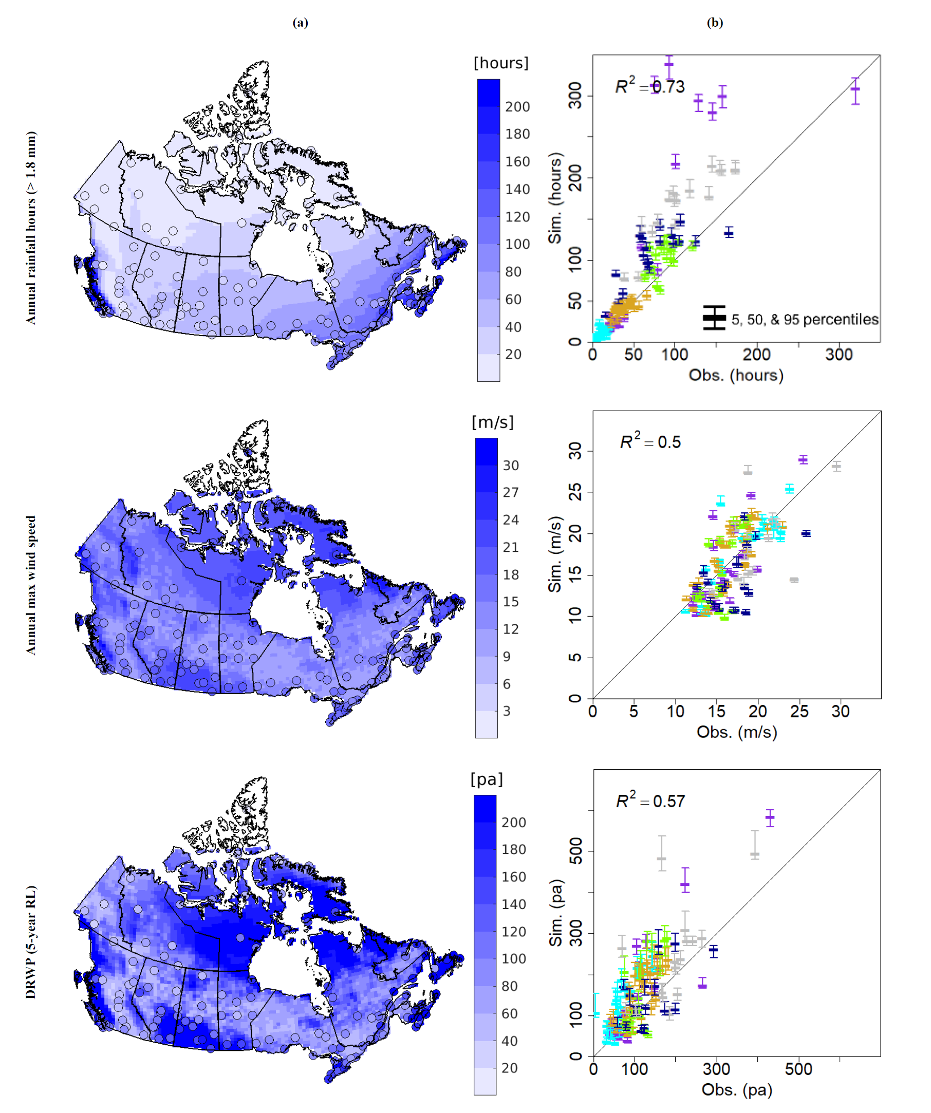
Projected changes to design (5-year return period) DRWPs and their internal variability are quantified using the CanESM2-CanRCM4 LE. Values are presented at different levels of future global mean temperature change above the 1986-2016 baseline. CanRCM4 LE projects a general increase in future design DRWPs over most regions of Canada (Figure 5.6). The spatial extent and relative magnitude of the increases tend to increase as global warming levels increase. On average, CanRCM4 LE projections of design DRWPs show +5 ~ +22% increases for the six Canadian regions at +3°C global warming level. British Columbia and North regions display larger increases compared to the other regions (Table 5.3). In particular, interquartile ranges of the design DRWPs for British Columbia and North regions exclude the zero-change line when global warming levels are +1°C and +2°C, respectively, relative to the baseline period (Figure 5.7).
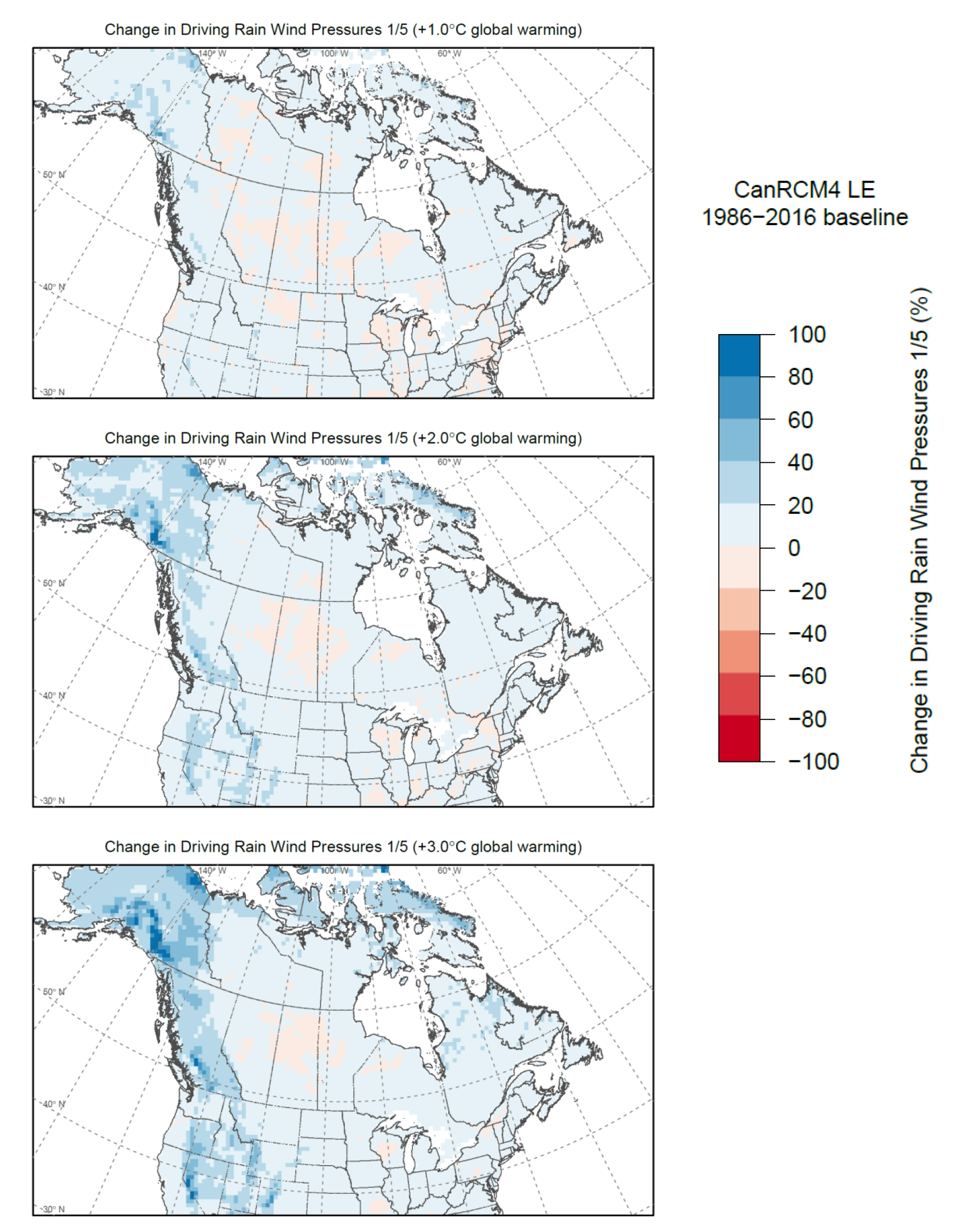
Table 5.3: Projected changes to 5-year return period DRWP for locations approximating Table C-2 locations in six Canadian regions and Canada as a whole for +1°C, +2°C, and +3°C global warming levels with respect to the 1986-2016 baseline period. Values represent the ensemble projection (25th percentile, 75th percentile) calculated from CanRCM4 LE.
| Change in driving rain wind press. 1/5 [%] | Global warming level | ||
|---|---|---|---|
| Region | +1°C | +2°C | +3°C |
| British Columbia | 6.7 (1.1, 13.2) | 11.9 (5.6, 19.2) | 15.1 (9.3, 22.7) |
| Prairies | 1.1 (-5.1, 8.1) | 4.5 (-3.8, 12.9) | 5.8 (-2.8, 15.7) |
| Ontario | 2.0 (-3.6, 8.4) | 5.4 (-1.8, 11.6) | 10.0 (2.4, 17.8) |
| Quebec | 2.6 (-3.4, 7.9) | 4.1 (-1.4, 12.5) | 6.6 (-0.2, 13.2) |
| Atlantic | 4.2 (-1.9, 9.5) | 6.5 (-0.1, 13.3) | 8.3 (1.7, 15.2) |
| North | 7.7 (-0.8, 16.9) | 13.5 (4.3, 24.2) | 22.0 (11.2, 30.9) |
| Canada | 2.8 (-2.9, 9.2) | 5.9 (-0.7, 13.4) | 9.0 (1.8, 16.8) |
CanRCM4 LE projects increases in the future frequency of rainfall > 1.8 mm/hr across Canada, reflecting the combined effects of increases in future total precipitation amounts and more frequent cold season (autumn-spring) rainfall caused by increases in air temperature (Figure 5.8). The spatial pattern of projected changes to rainfall (> 1.8 mm/hr) frequency is in good agreement with projected changes in design DRWP (shown in Figure 5.6 at the +2 °C global warming level), with larger increases over British Columba, the North, and northern parts of Quebec. Therefore, there is evidence that increases in future rainfall frequency is the main contributor to the projected increases in future design DRWP. Consequently, spatial patterns of projected changes in design DRWPs are quite different from those for design wind pressures presented in Figure 5.1 and Figure 5.2 particularly over British Columbia and North regions. Moreover, relative projected changes to design DRWPs are larger than those of design wind pressures.
(a) Annual mean air temperature (2 m) [°C]
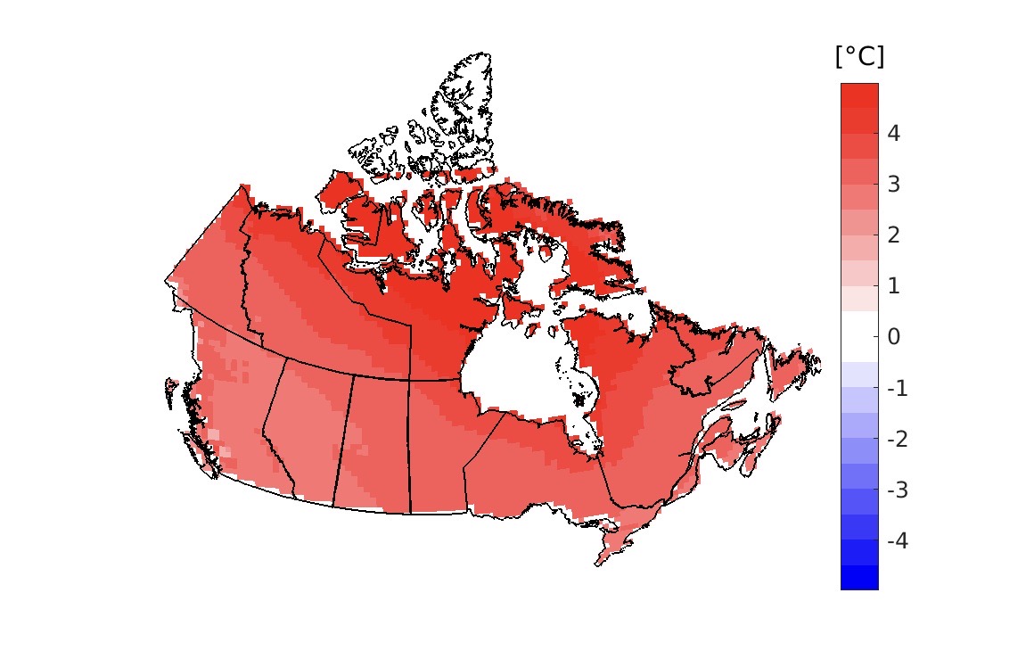
(b) Annual total precipitation [%]
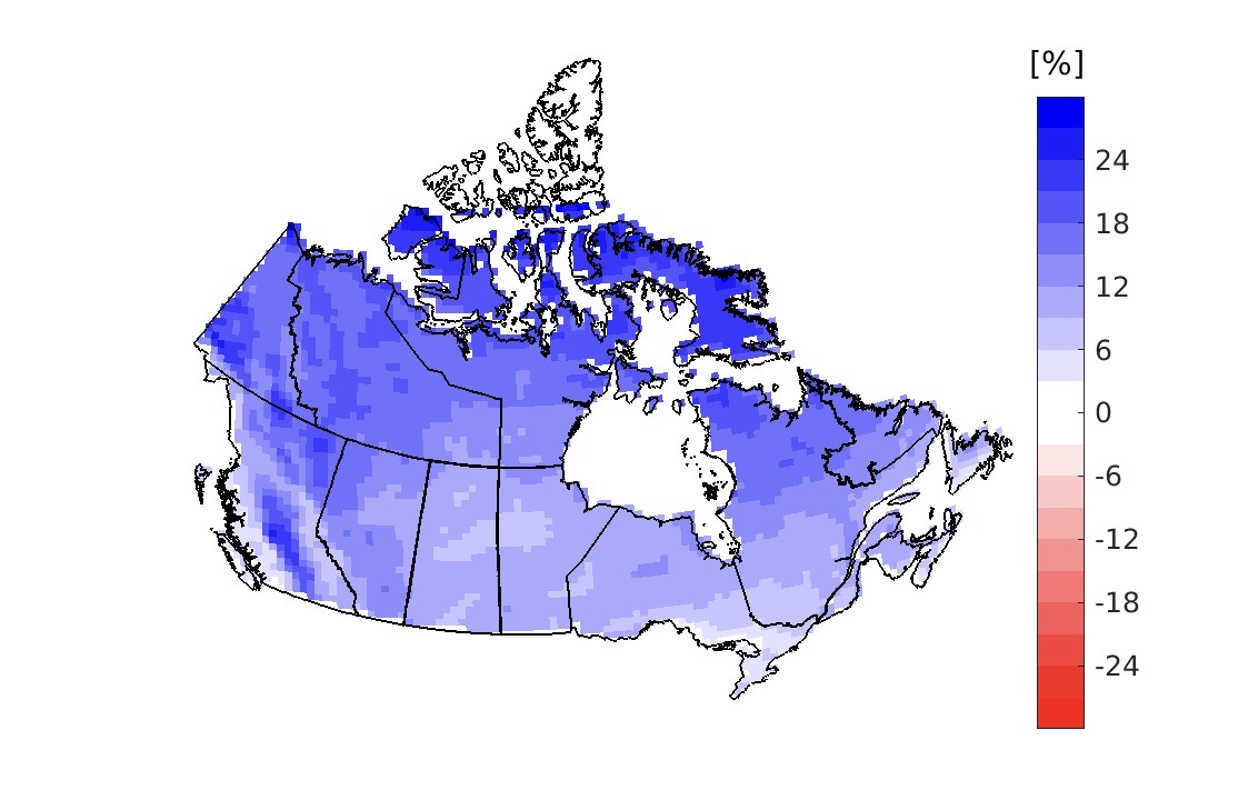
(c) Autumn-spring total rainfall [%]
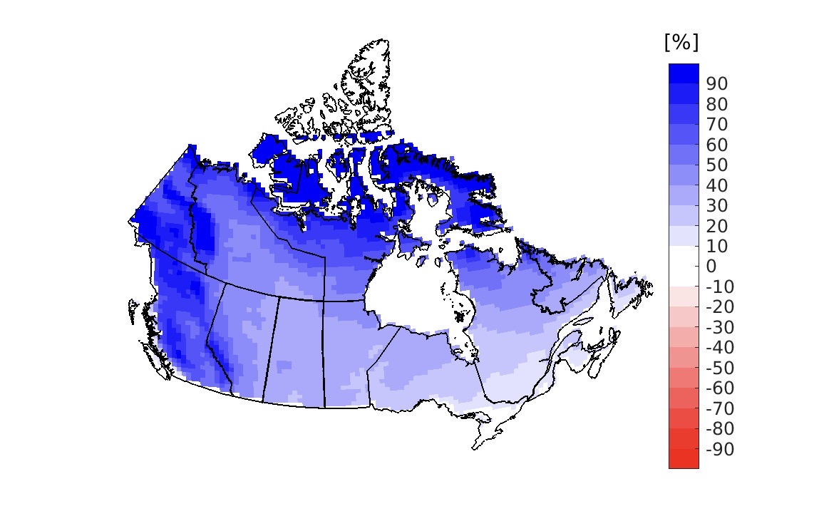
(d) Annual rainfall (>1.8 mm) hours [%]
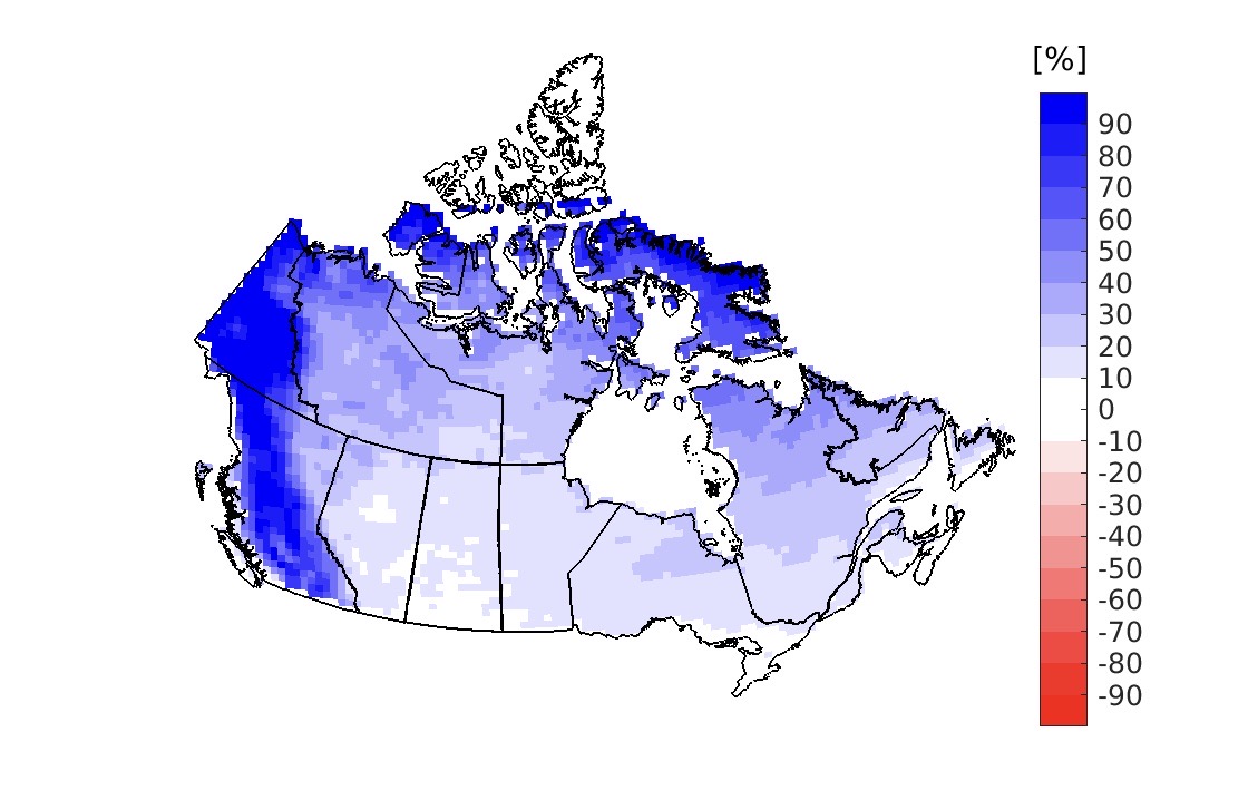
The link with temperature and corresponding increase in the proportion of precipitation events that occur as rainfall leads to medium confidence that DRWPs will increase. There is nevertheless very low confidence in the pattern and magnitude of projected DRWP changes due high uncertainty from multiple sources in rainfall and wind speed projections. Internal variability in rainfall and wind speeds leads to large interquartile ranges in the CanRCM4 projected DRWP changes for all Canadian regions and future periods (Table 5.3 and Figure 5.7). As mentioned before in the context of wind extremes, additional uncertainty in the projected changes stem from difficult to quantify modelling uncertainties that are reflected in the difficulty in simulating extratropical cyclones in GCMs and RCMs, and because some key processes such as small-scale convective wind storms are not represented. In addition, there is considerable model related uncertainty in the response of model simulated winds to external forcing. There are also many model related uncertainties that pertain to the rainfall aspect of DRWP (section 4.1 and section 4.2). For example, although the CanRCM4 pattern of rainfall changes (section 4.1.2; Figure 4.1) corresponds with the enhanced regional changes in DRWP, this pattern itself should be considered to have much lower confidence because of the paucity of research on projected rainfall changes and its regional variations using different models.
5.2.3 Interpretation
DRWP is a Tier 3 variable that combines changes in the frequency of heavy rainfall with changes in high winds.
As assessed above, there is medium confidence overall that DRWP will increase. Projected increases are driven primarily by increases in the frequency of future rainfall (> 1.8 mm/hr) occurrence due to combined increases in air temperature and precipitation amounts. Projected changes in temperature and precipitation, and hence rainfall, are relatively well understood over Canada, as compared to the changes in mean and extreme wind speeds. As is the case for wind loads, values of NS ratio for DRWP tend to be close to one at all global warming levels. Nevertheless, even in the absence of changes to wind speed and co-occurrence of wind and precipitation, increases in the frequency of rainfall will lead to increases in DRWP.
In contrast, there is very low confidence in the projected magnitude of change. Regionally, CanRCM4 LE projects larger increases in DRWP over British Columbia and the North, with emergence of the forced signal from internal variability at global warming levels that exceed +1°C and +2°C respectively. There is, however, a paucity of research and thus it is not possible to assess the robustness of these results across different climate modelling systems.
Nevertheless, increases in DRWP could be an emerging risk for existing buildings designed based on historical DRWP data. Projected changes at locations approximating Table C-2 locations are therefore provided in Appendix 1.2 from CanRCM4 LE for each global warming level. It is not possible to assess a level of confidence for these place-specific projections, but they are offered so that they can be used by practitioners to explore potential future scenarios and as an adjunct for risk analysis.
6. Snow and ice
6.1 Snow loads
6.1.1 Assessment
The snow load elements of NBCC Table C-2 are used to account for the gravitational loads induced by snow accumulation on the roofs of buildings. Total snow load is determined by combining two components: ground snow load and an associated rain load. Ground load is converted to a roof load via a basic factor, an accumulation factor that accounts for drifts, a slope factor, and a wind or exposure factor, before rain load is added. As the amount of snow on roofs is not monitored routinely, ground snow load is used as the reference from which the roof snow load is estimated. The associated rain load considers wet snow conditions caused by rain-on-snow events; however, it is constrained not to exceed the design ground snow load and is usually smaller than 10% of the ground snow load component.
Areal snow covered extent (SCE) and snow water equivalent (SWE) are key characteristics of the ground snow load, whose accumulation and ablation respond to both temperature and precipitation. Annual maximum values of accumulated SWE on the ground are used to determine design ground snow loads. Unlike SCE, SWE takes into account both snow depth and density. In the NBCC, the design ground snow load is associated with the 50-year return period as estimated from the Gumbel distribution fitted to the annual maximum values.
The CCCR (Bush and Lemmen, 2019)Reference 3 assessed historical trends and future projections of SCE and SWE in Canada. The portion of the year with snow cover has decreased across most of Canada by 5% to 10% per decade since 1981, due to later snow onset and earlier spring melt (very high confidence). The observed seasonal snow accumulation has also decreased by 5% to 10% per decade, with the exception of southern Saskatchewan, and parts of Alberta and British Columbia (increases of 2% to 5% per decade). Based on climate model projections, it is very likely under all emissions scenarios that snow cover duration will decline to mid-century over Canada due to increases in surface air temperature. Differences in spring snow cover projections between emissions scenarios emerge by end of century, with stabilized snow loss for the RCP4.5 emissions scenario due to stabilization of radiative forcings in 2080 and associated stabilization of air temperature over Canada (Figure 2.2), but continued snow loss under the RCP 8.5 emissions scenario. A reduction of 5% to 10% per decade in seasonal snow accumulation (through 2050) is projected over much of southern Canada. In contrast, only small changes in snow accumulation are projected over northern regions of Canada because increases in winter precipitation are expected to offset a shorter snow accumulation period (medium confidence).
More generally, international assessments have concluded that there is very high confidence that SCE has decreased in the Northern Hemisphere, especially in spring (IPCC, 2013)Reference 4. According to the IPCC (2013)Reference 4, the Northern Hemisphere spring SCE decreased by 1.6% per decade over the 1967-2012 period. Recent research has attributed the observed decrease in spring SCE in the high latitudes of Northern Hemisphere to human influence (Rupp et al., 2013Reference 101; Najafi et al., 2016Reference 102) and has shown that SCE decrease is closely linked to a shortening of the seasonal snow cover duration (Brown and Mote, 2009)Reference 103.
International assessments indicate high confidence that spring SCE over the Northern Hemisphere will be substantially lower by the end of this century if anthropogenic climate forcing growth is uncontrolled (IPCC, 2013)Reference 4. Future reductions of SCE, particularly over southern Canada in spring, are also projected by CMIP3 (Roesch, 2006Reference 104; Brown and Mote, 2009Reference 103) and CMIP5 GCMs (Brutel-Vuilmet et al., 2013Reference 105, Mudryk et al., 2018Reference 106). However, there is low confidence in the projected magnitude of SCE reductions over the Northern Hemisphere as snow processes in global climate models are heavily simplified (IPCC, 2013)Reference 4.
There has also been considerable research on observed and projected changes in snow amount. For example, based on in situ observations, decreases in spring snow depth or SWE have been reported over China (Ma and Qin, 2012)Reference 107 and the European Alps (Marty and Meister, 2012)Reference 108. Studies also have reported decreases in spring SWE during the last three decades over the Northern Hemisphere based on satellite-based datasets (e.g., Luojus et al. 2011Reference 109; Gan et al. 2013Reference 110). Decreases in spring SWE inferred from observationally constrained analyses have been attributed to anthropogenic influence over the northern half (> 45°) of Northern Hemisphere (Jeong et al., 2017)Reference 111 and in southern British Columbia (Najafi et al., 2017)Reference 112.
The IPCC (2013)Reference 4 reported that global warming will decrease SWE as the climate continues to warm both by changing snow to rain and by increasing snowmelt. On the other hand, increases in precipitation will result in increases in snow amounts over much of the northern high latitudes during winter months because temperatures will still remain below freezing. Based on both CMIP3 (Räisänen, 2008)Reference 113 and CMIP5 models (Brutel-Vuilmet et al., 2013)Reference 105, annual maximum SWE may increase somewhat in the coldest regions, but it is expected to decrease strongly in the southern limit of the seasonally snow-covered area by the end of this century, although the timing of these projected changes is highly dependent on emission scenario.
Overall, there is medium confidence that annual maximum SWE, and hence the snow component of ground snow load, will either increase or exhibit little change in the northern high latitudes and decrease further south, due to the competing factors of temperature and precipitation increases. However, given the low confidence in magnitude of SCE decreases, in combination with additional uncertainty in SWE projections, there is very low confidence in the projected magnitude of changes in ground snow loads in Canada.
6.1.2 Targeted research
The assessment of future changes in snow accumulation in the CCCR (Bush and Lemmen, 2019)Reference 3 is based on GCM projections for fixed time periods under different emission scenarios. As described in chapter 1, the approach recommended for B&CPI is instead to provide regional changes tied to fixed levels of global warming, rather than for fixed time periods under different scenarios, as this substantially reduces emissions scenario dependence over much of the current century.
Projected changes to design snow loads (50-year return period) and their internal variability are quantified using daily outputs of SWE obtained directly from CanESM2-CanRCM4 LE simulations. The Gumbel distribution is fitted via the method of moments to the annual maxima of daily SWE amounts for 31-year periods associated with different levels of global warming; values are thus calculated directly from SWE, rather than from snow depth and snow density as in the NBCC. Results are provided at specific levels of future global mean temperature change (e.g., +1, +2, and +3°C) above the 1986-2016 baseline level.
CanRCM4 LE projects decreases in future design snow loads over southern regions of Canada. The spatial extent and relative magnitude of the decreases tend to increase with the level of global warming (see Figure 6.1 and Figure 6.2). This is primarily caused by increases in future surface air temperatures, which lead to overall decreases in ground snow accumulations and annual maximum SWE due to delayed snow onset and earlier snowmelt as well as more frequent snowmelt during the snow season. Conversely, projected changes to design snow loads show some increases over the North (Table 6.1). This is mainly due to continued increases in precipitation falling as snow in the future. However, the relative magnitude of the projected changes over this region is small, e.g., roughly +5% for +3°C global warming level relative to the baseline period, as increases in winter precipitation are offset by a shorter snow accumulation period.
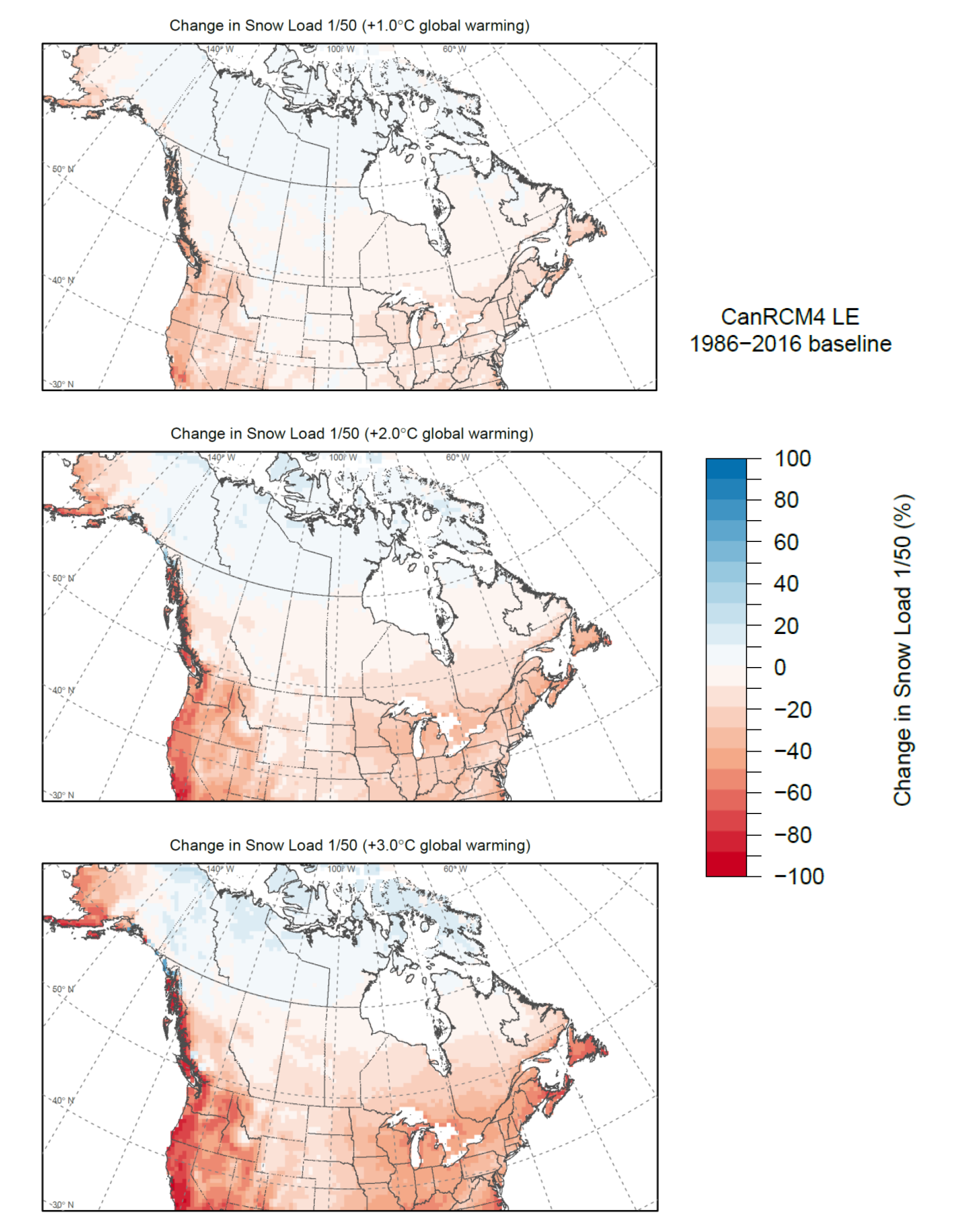
Table 6.1: CanRCM4 LE projected changes in design snow loads (SLs) for locations approximating Table C-2 locations in six Canadian regions and Canada as a whole for +1.0°C, +2.0°C, and +3.0°C global warming levels with respect to the 1986-2016 baseline period. Values represent the ensemble projection (25th percentile, 75th percentile) calculated from CanRCM4 LE.
| Change in snow load 1/50 [%] | Global warming level | ||
|---|---|---|---|
| Region | +1°C | +2°C | +3°C |
| British Columbia | -22.0 (-35.4, -8.7) | -39.2 (-55.2, -24.9) | -55.8 (-68.9, -45.2) |
| Prairies | -1.6 (-10.4, 8.1) | -5.5 (-16.6, 5.6) | -12.6 (-21.4, -2.5) |
| Ontario | -18.3 (-27.2, -7.1) | -31.6 (-42.1, -21.4) | -41.9 (-52.1, -34.1) |
| Quebec | -13.7 (-22.9, -4.4) | -27.6 (-35.3, -18.8) | -40.4 (-49.2, -34.9) |
| Atlantic | -25.2 (-34.1, -14.8) | -43.0 (-52.3, -35.8) | -61.7 (-68.0, -57.0) |
| North | 4.0 (-1.9, 9.6) | 5.4 (-0.4, 11.9) | 5.4 (0.2, 12.5) |
| Canada | -14.8 (-23.0, -4.6) | -28.1 (-36.7, -18.8) | -40.7 (-49.8, -32.5) |
While projected changes to basic characteristics of rain-on-snow events, such as occurrence frequency and total amounts, have been investigated by Jeong and Sushama (2018b)Reference 31 using a different Canadian RCM, CRCM5, which was also run at 0.44° grid spacing, studies for extreme rain-on-snow amounts have not been conducted for Canada. When compared to projected changes in the snow component, CanRCM4 LE simulations suggest smaller relative changes to the rain component with much larger internal variability (Figure 6.3). However, as mentioned above, the rain component is usually smaller than 10% of the ground snow load component and its magnitude is limited to be no more than the ground snow load. Nevertheless, overall uncertainty about compound rain/snow-on-ground processes is high. Finally, as a supplement, projected changes to the mean and coefficient of variation of the snow load components are provided in Table S6.1 and Table S6.2, respectively.
Table S6.1: Projected changes to mean of snow load (SLs) (top panel), rain load (SLr) (middle panel), and ice thickness (bottom panel) variables for locations approximating Table C-2 locations in six Canadian regions and Canada as a whole for global warming levels from +0.5°C to +3.5°C with respect to the 1986-2016 baseline period. Values represent the ensemble projection (25th percentile, 75th percentile) calculated from CanRCM4 LE.
| Change in snow load mean [%] | Global warming level | ||||||
|---|---|---|---|---|---|---|---|
| Region | +0.5°C | +1°C | +1.5°C | +2°C | +2.5°C | +3°C | +3.5°C |
| British Columbia | -20.2 (-25.1, -12.2) | -34.3 (-41.4, -25.1) | -46.3 (-54.9, -37.7) | -56.9 (-62.8, -47.9) | -64.8 (-71.4, -58.1) | -71.7 (-77.8, -66.2) | -77.0 (-81.2, -71.0) |
| Prairies | -2.2 (-6.6, 2.5) | -3.8 (-10.1, 2.2) | -7.3 (-14.4, -1.1) | -11.7 (-18.3, -5.1) | -16.4 (-22.4, -10.5) | -21.4 (-26.8, -15.1) | -26.4 (-32.4, -20.5) |
| Ontario | -12.4 (-17.9, -6.4) | -22.4 (-28.8, -15.1) | -33.5 (-39.6, -26.1) | -41.4 (-47.0, -34.0) | -49.9 (-54.9, -43.8) | -56.5 (-61.8, -50.7) | -63.1 (-67.9, -58.5) |
| Quebec | -11.9 (-17.8, -6.3) | -21.0 (-28.1, -12.8) | -31.3 (-35.8, -23.6) | -38.5 (-44.0, -30.8) | -47.0 (-52.9, -41.7) | -53.1 (-58.8, -48.0) | -60.2 (-63.4, -56.3) |
| Atlantic | -20.1 (-25.8, -14.6) | -34.0 (-40.2, -27.7) | -46.8 (-51.9, -40.1) | -58.0 (-62.2, -53.3) | -67.6 (-70.8, -63.9) | -75.2 (-78.0, -71.8) | -80.8 (-84.0, -78.0) |
| North | 1.7 (-0.3, 4.1) | 2.5 (-0.4, 5.7) | 3.2 (0.0, 6.2) | 3.4 (0.3, 6.6) | 3.1 (-0.2, 7.6) | 3.2 (-0.2, 7.0) | 1.4 (-1.7, 4.6) |
| Canada | -11.7 (-17.2, -5.6) | -21.3 (-27.3, -13.6) | -31.8 (-37.1, -25.0) | -40.0 (-44.7, -33.0) | -48.5 (-53.3, -42.4) | -55.0 (-60.2, -49.2) | -61.3 (-65.6, -56.6) |
| Change in rain load mean [%] | Global warming level | ||||||
|---|---|---|---|---|---|---|---|
| Region | +0.5°C | +1°C | +1.5°C | +2°C | +2.5°C | +3°C | +3.5°C |
| British Columbia | 0.5 (-3.0, 3.8) | -1.6 (-4.9, 2.3) | -5.9 (-10.8, -1.8) | -13.6 (-18.1, -7.9) | -24.3 (-28.6, -20.1) | -35.2 (-38.3, -32.6) | -46.6 (-50.3, -43.4) |
| Prairies | 4.0 (-3.6, 11.3) | 8.0 (-2.4, 18.9) | 11.7 (1.2, 24.1) | 14.9 (3.0, 27.4) | 18.1 (7.2, 30.4) | 19.4 (8.1, 32.1) | 21.4 (9.2, 33.5) |
| Ontario | -6.3 (-11.0, -1.0) | -13.3 (-20.0, -5.6) | -22.1 (-29.5, -15.7) | -31.3 (-36.5, -25.3) | -39.4 (-45.3, -33.6) | -46.5 (-51.1, -40.8) | -53.3 (-57.3, -49.0) |
| Quebec | -2.3 (-7.2, 1.1) | -7.3 (-12.7, -0.8) | -13.5 (-18.9, -6.2) | -20.1 (-26.2, -13.6) | -26.8 (-31.9, -21.2) | -33.8 (-38.0, -28.9) | -41.0 (-45.3, -35.8) |
| Atlantic | -12.9 (-16.6, -7.2) | -23.1 (-29.2, -16.8) | -34.2 (-41.2, -28.1) | -46.1 (-52.1, -40.4) | -57.8 (-61.7, -53.5) | -66.7 (-71.1, -62.1) | -73.5 (-77.2, -70.1) |
| North | 3.2 (-4.6, 10.9) | 6.3 (-3.6, 16.2) | 8.4 (-1.8, 21.7) | 13.2 (1.6, 24.3) | 17.0 (5.2, 29.5) | 20.4 (9.7, 33.7) | 25.5 (14.3, 37.2) |
| Canada | -2.7 (-7.5, 1.2) | -7.3 (-12.9, -0.8) | -13.6 (-18.9, -6.9) | -20.7 (-26.3, -15.4) | -28.4 (-33.2, -22.9) | -35.8 (-40.4, -30.6) | -42.8 (-47.5, -38.6) |
| Change in ice thickness mean [%] | Global warming level | ||||||
|---|---|---|---|---|---|---|---|
| Region | +0.5°C | +1°C | +1.5°C | +2°C | +2.5°C | +3°C | +3.5°C |
| British Columbia | 2.0 (-7.9, 20.7) | 1.0 (-12.6, 32.4) | 2.1 (-13.6, 34.0) | -1.0 (-12.7, 25.5) | -6.3 (-17.4, 16.0) | -11.3 (-28.3, 14.8) | -14.0 (-29.2, 14.1) |
| Prairies | 13.6 (-4.8, 34.9) | 25.5 (0.0, 57.7) | 36.8 (9.8, 75.8) | 43.8 (16.8, 88.7) | 50.4 (24.6, 98.0) | 59.6 (28.7, 105.9) | 63.2 (28.7, 115.7) |
| Ontario | -2.1 (-14.5, 10.6) | -3.3 (-19.1, 14.4) | -7.8 (-24.0, 10.0) | -13.5 (-28.8, 5.1) | -21.8 (-36.6, -8.2) | -31.1 (-43.0, -17.7) | -40.8 (-53.6, -27.9) |
| Quebec | 2.5 (-7.7, 13.3) | 1.8 (-10.6, 16.6) | 0.8 (-14.7, 19.5) | -0.7 (-12.8, 16.3) | -4.0 (-18.3, 11.7) | -7.2 (-21.8, 10.1) | -16.3 (-30.1, -1.8) |
| Atlantic | -7.2 (-16.0, 4.8) | -13.8 (-25.6, 5.3) | -25.5 (-35.8, -7.5) | -37.5 (-46.8, -20.9) | -48.5 (-57.6, -37.3) | -57.5 (-65.7, -50.3) | -66.6 (-73.8, -59.0) |
| North | 10.3 (-8.1, 35.0) | 15.8 (-9.4, 67.5) | 24.5 (-2.4, 88.5) | 37.7 (2.6, 98.8) | 56.0 (15.4, 123.0) | 67.8 (15.9, 138.6) | 86.4 (30.6, 165.6) |
| Canada | 1.3 (-9.4, 13.5) | 1.0 (-12.8, 17.5) | 0.0 (-15.5, 17.5) | -1.9 (-18.7, 15.0) | -6.2 (-20.5, 11.7) | -11.3 (-26.4, 8.5) | -18.0 (-32.8, -1.8) |
Table S6.2: Projected changes to coefficient of variation (CoV) of snow load (SLs) (top panel), rain load (SLr) (middle panel), and ice thickness (bottom panel) variables for locations approximating Table C-2 locations in six Canadian regions and Canada as a whole for global warming levels from +0.5°C to +3.5°C with respect to the 1986-2016 baseline period. Values represent the ensemble projection (25th percentile, 75th percentile) calculated from CanRCM4 LE.
| Change in snow load CoV [%] | Global warming level | ||||||
|---|---|---|---|---|---|---|---|
| Region | +0.5°C | +1°C | +1.5°C | +2°C | +2.5°C | +3°C | +3.5°C |
| British Columbia | 6.3 (-4.3, 20.7) | 13.6 (-2.8, 30.8) | 23.4 (3.2, 38.6) | 30.3 (13.9, 54.7) | 45.8 (26.5, 72.6) | 61.3 (47.0, 83.0) | 84.4 (59.3, 119.5) |
| Prairies | 2.2 (-5.9, 11.9) | 4.5 (-7.0, 18.2) | 7.7 (-4.7, 22.6) | 11.3 (-3.2, 26.8) | 14.6 (0.0, 31.0) | 20.2 (5.7, 36.6) | 27.3 (10.4, 44.0) |
| Ontario | 6.0 (-3.0, 17.1) | 8.3 (-4.2, 24.8) | 15.5 (0.9, 34.2) | 24.8 (11.0, 43.8) | 35.9 (21.0, 57.4) | 48.7 (30.1, 68.5) | 59.4 (38.5, 81.1) |
| Quebec | 8.5 (0.3, 17.9) | 12.9 (-0.5, 28.7) | 21.5 (6.5, 35.9) | 30.1 (16.2, 48.4) | 37.9 (20.8, 53.6) | 46.8 (30.3, 65.4) | 53.0 (36.9, 69.7) |
| Atlantic | 10.1 (-2.1, 22.1) | 20.0 (4.8, 38.1) | 35.0 (18.4, 58.4) | 53.5 (31.0, 76.7) | 69.2 (46.0, 93.5) | 88.5 (59.5, 112.5) | 111.2 (74.1, 135.5) |
| North | 1.4 (-6.8, 10.0) | 3.0 (-8.9, 14.9) | 3.2 (-8.5, 17.5) | 4.9 (-7.1, 17.0) | 5.5 (-5.2, 19.1) | 7.6 (-3.5, 19.9) | 10.8 (-1.8, 25.0) |
| Canada | 6.3 (-3.2, 17.0) | 9.4 (-3.4, 25.7) | 17.1 (2.1, 34.4) | 26.7 (11.9, 44.2) | 35.6 (19.3, 55.2) | 46.3 (26.5, 65.7) | 54.1 (36.7, 76.7) |
| Change in rain load CoV [%] | Global warming level | ||||||
|---|---|---|---|---|---|---|---|
| Region | +0.5°C | +1°C | +1.5°C | +2°C | +2.5°C | +3°C | +3.5°C |
| British Columbia | 2.3 (-6.5, 12.2) | 4.5 (-10.5, 20.3) | 16.3 (-2.3, 31.5) | 31.3 (18.2, 51.1) | 59.8 (42.8, 87.7) | 81.1 (58.8, 109.8) | 110.6 (78.1, 139.7) |
| Prairies | -4.1 (-13.1, 5.7) | -7.7 (-19.8, 7.3) | -10.6 (-22.5, 5.1) | -13.6 (-25.2, 1.8) | -15.7 (-26.9, 0.0) | -17.8 (-29.5, -3.6) | -18.4 (-29.9, -4.9) |
| Ontario | 5.6 (-3.5, 15.3) | 10.1 (-4.6, 23.3) | 17.4 (1.4, 32.7) | 27.9 (13.2, 44.6) | 40.4 (22.3, 58.1) | 52.9 (31.0, 70.6) | 63.0 (40.0, 84.6) |
| Quebec | 3.3 (-4.9, 11.6) | 5.7 (-7.4, 17.6) | 12.2 (-1.4, 24.1) | 23.0 (9.0, 36.4) | 34.8 (18.0, 49.7) | 41.9 (25.5, 58.9) | 53.8 (34.2, 72.8) |
| Atlantic | 12.5 (1.8, 22.4) | 26.4 (12.2, 41.8) | 43.4 (26.6, 59.2) | 61.8 (40.6, 82.0) | 85.1 (55.5, 103.8) | 103.4 (75.4, 125.8) | 133.7 (94.9, 157.1) |
| North | -0.6 (-9.9, 10.3) | -2.2 (-15.4, 12.2) | -3.7 (-17.3, 12.8) | -4.8 (-18.6, 9.1) | -6.3 (-20.2, 6.8) | -9.6 (-22.0, 4.8) | -11.7 (-24.1, 4.1) |
| Canada | 3.1 (-5.6, 12.5) | 5.8 (-8.0, 19.1) | 12.2 (-2.3, 26.2) | 21.5 (6.1, 39.5) | 30.6 (13.4, 49.7) | 41.3 (21.3, 61.2) | 49.7 (31.7, 72.1) |
| Change in ice thickness CoV [%] | Global warming level | ||||||
|---|---|---|---|---|---|---|---|
| Region | +0.5°C | +1°C | +1.5°C | +2°C | +2.5°C | +3°C | +3.5°C |
| British Columbia | -2.4 (-11.4, 9.1) | -4.8 (-15.8, 12.9) | -0.7 (-16.4, 17.9) | 1.1 (-11.2, 20.4) | 6.5 (-8.0, 26.4) | 11.2 (-2.0, 36.3) | 20.8 (1.8, 46.8) |
| Prairies | -6.8 (-17.6, 4.2) | -11.6 (-25.6, 3.0) | -15.4 (-29.6, 0.2) | -17.7 (-32.0, -3.1) | -19.1 (-31.0, -5.2) | -20.6 (-33.4, -5.3) | -20.1 (-32.7, -6.1) |
| Ontario | 3.3 (-5.7, 15.3) | 8.2 (-4.7, 23.5) | 14.2 (-0.3, 33.5) | 26.5 (10.7, 44.9) | 37.5 (17.9, 58.5) | 52.7 (31.3, 78.6) | 64.6 (48.5, 92.5) |
| Quebec | -0.2 (-8.6, 11.0) | 2.4 (-11.7, 16.6) | 7.5 (-8.3, 20.7) | 10.8 (-2.2, 26.2) | 18.5 (3.1, 36.4) | 25.2 (5.9, 45.4) | 31.3 (11.5, 49.8) |
| Atlantic | 5.7 (-4.0, 17.9) | 12.6 (-3.5, 29.6) | 26.0 (7.7, 45.8) | 37.8 (21.7, 62.1) | 51.4 (31.6, 85.0) | 70.5 (50.1, 102.6) | 94.8 (68.0, 132.9) |
| North | -3.7 (-16.1, 7.2) | -5.2 (-20.6, 9.1) | -10.6 (-27.5, 7.2) | -15.1 (-33.0, 4.5) | -22.1 (-39.5, -4.1) | -27.5 (-46.0, -10.8) | -34.0 (-48.5, -22.4) |
| Canada | 0.3 (-9.3, 11.7) | 2.8 (-11.7, 18.0) | 6.6 (-9.7, 23.0) | 11.3 (-3.4, 27.1) | 18.5 (2.7, 36.4) | 24.5 (6.6, 45.4) | 31.3 (11.0, 51.8) |
Confidence in both the snow load and associated rain load projections is very low despite medium confidence in the large-scale pattern of projected snow load changes, with decreases in southern Canada, and little change or modest increases in the North. There is very low confidence in projected changes in snow cover extent, also very little confidence in the differentiations of regions with projected decreases, and those with little change or modest increases. In addition, model uncertainty associated with the GCMs and RCMs, their land surface sub-models, and their use of highly simplified snow models, leads to very high, difficult to quantify, model uncertainty. This is further complicated for rain loads since very little research has been done to assess the ability of models to simulate rain-on-snow events and whether the processes and synoptic situations that produce such events are adequately represented in models.
6.1.3 Interpretation
Snow load is a Tier 3 variable. Projected changes in snow and rain components at locations approximating Table C-2 locations are provided in Appendix 1.2. Values are based on projections from CanRCM4 LE. Overall, spatial patterns of CanRCM4 LE projected changes in the snow component over Canada are consistent with findings from global climate models for SCE (e.g., Peacock, 2012Reference 114; Brutel-Vuilmet et al., 2013Reference 105; Mudryk et al., 2018Reference 106), snow depth (Peacock, 2012)Reference 114, and annual maximum SWE (e.g., Räisänen, 2008Reference 113; Brutel-Vuilmet et al., 2013Reference 105), as well as from CRCM5 simulations of snow loads (Jeong and Sushama, 2018a)Reference 89. Given this consistency, as well the linkages between changes in temperature, precipitation, and SWE, there is as also noted above medium confidence in the spatial pattern of decreases to the snow component of snow loads projected by CanRCM4 LE in the south and possible increases in the North. The magnitude of change is more uncertain (very low confidence) due to the role of internal variability, as represented by the range in Figure 6.2, as well as a wide range of difficult to quantify model uncertainties. Values of NS ratio for the snow component of total snow load typically exceed 0.5 until the +2.5°C global warming level indicating substantial uncertainty due to internal variability. Furthermore, greater uncertainty is expected in areas with complex terrain that are not resolved at the spatial resolution of CanRCM4 (e.g., Terzago et al., 2017)Reference 115. There is also very low confidence about future projections of the rain component of snow load, due in large part to high internal variability, as well as the compound nature of the variable – rain must occur coincident with the presence of snow on the ground; values of NS ratio typically exceed 0.5 at all global warming levels – and model uncertainties that affect the presence or absence of snow on the ground, precipitation in general, and representation of processes responsible for the occurrence of rainfall in the cold.
Decreases in the future ground component of design snow loads projected by CanRCM4 LE for southern Canada are consistent with findings for SCE, snow depth, SWE, and snow loads from previous GCM and RCM projections and process understanding. There is therefore medium confidence that the snow component of design snow loads will decrease with warming in all regions except the Prairies (low confidence in decreases) and the North (low confidence that there will be either no change or a modest increase). There is very low confidence in the magnitude of the projected changes in all regions.
6.2 Ice accretion loads
6.2.1 Assessment
Ice accretion loads are specified to take into account ice accretion on all exposed surfaces of highway bridges, such as superstructure members, structural supports, traffic signals, luminaires, railings, sign panels, bridge girders, and solid barriers. Atmospheric ice accretion is mainly caused by freezing precipitation during ice storms, while freezing precipitation generally occurs when precipitation falls through warm layers aloft (> 0°C) and then arrives at a sub-freezing surface layer (mostly in the range -10°C to approximately 0°C) (Cortinas et al., 2004)Reference 116. Ice accretion thickness is affected by other variables, including surface wind speed and surface air temperature (Chaîné and Castonguay, 1974)Reference 117. In the CHBDC, the design ice accretion load is associated with the 20-year return period as estimated from the Gumbel distribution fitted to the annual maximum ice thickness series.
The measurement and simulation of freezing precipitation is challenging because it is often mixed with other precipitation types (e.g., rain, snow, and ice pellets) and it occurs with lower frequency than rainfall and snow due to the narrow range of upper level and surface air temperatures that control its formation. Nevertheless, changes in the frequency of freezing precipitation during the recent decade compared to the late 20th century have been evaluated by Groisman et al. (2016)Reference 118 over North America based on weather station data. They found decreases in the frequency of freezing precipitation over southeastern US, but increases over northern parts of North America.
A few studies have investigated how freezing precipitation could evolve under climate change. Based on the third-generation Canadian Coupled Climate Model (CGCM3, a predecessor to CanESM2), Lambert and Hansen (2011)Reference 119 found a poleward shift of future freezing precipitation at the end of this century due to future surface temperature increases and consequent poleward shift of the 0°C isotherm. However, they noted that CGCM3’s coarse resolution might not be sufficient to accurately project regional changes in freezing precipitation. Klima and Morgan (2015)Reference 120 investigated climate change impacts on ice storm occurrences over southeastern Canada and eastern US, based on an experiment using historical vertical temperature profiles combined with several upper level and surface temperature warming scenarios. They also found a poleward shift of future freezing precipitation with an increase in winter ice storm events, but overall decreases for the southern US.
RCMs, which generally represent the topography in more detail than do GCMs and sometimes also better represent the key processes leading to freezing precipitation, have recently been used to investigate historical freezing precipitation events. For instance, Bresson et al. (2017)Reference 121 showed that CRCM5 is able to reproduce the climatology of freezing rain and ice pellets in the Montréal region as well as the freezing-rain event that occurred in the region in January 1998. St.-Pierre et al. (2019)Reference 122 further assess the model over eastern Canada, noting generally good performance, although finding that bias in the frequency of freezing rain occurrence was resolution dependent, with overestimation of frequency when the model was run at 0.11° spatial resolution, but underestimation when run at a lower 0.44° spatial resolution. Moreover, RCMs have been used to quantify projected changes to freezing precipitation characteristics, such as frequency, intensity, extreme events, and geographical distribution. In particular, using CRCM5, Jeong et al. (2018)Reference 123 found general increases in the future monthly freezing precipitation frequency and amounts to the north from the future 0°C isotherm of monthly mean surface temperature, but general decreases to the south from the future freezing line, consistent with previous studies. Thus, consistent with Lambert and Hansen (2011)Reference 119, the placement of the 0°C isotherm at different levels of warming may give some indication of the direction and magnitude of changes in freezing precipitation. Nevertheless, overall confidence remains very low, given the complexity of the processes involved and the paucity of work involving models that are able to explicitly represent these processes.
The number of studies that have focused on projected changes to ice accretion loads and associated impacts on infrastructure is also very limited. Rezaei et al. (2016)Reference 124 evaluated changes in the reliability of electric transmission lines to changes in atmospheric ice accretion, based on a range of assumed changes in the mean and standard deviation of future ice accretion loads. They noted the need for local and regional scale climate change scenarios to complete a comprehensive risk analysis. Jeong et al. (2018)Reference 123 quantified changes to design ice accretion loads for overhead transmission lines for two future periods (i.e., 2041-2070 and 2071-2100) with respect to the 1976–2005 period over Canada, using simulations from CRCM5 driven by two GCMs (i.e., CanESM2 and the Max-Planck-Institut Earth System Model) for RCP 4.5 and 8.5 scenarios. They found broad increases in the design ice accretion loads for eastern Canada, scattered increases for south central and western Canada, and some decreases for the east coast and Great Lakes regions for the future periods.
While a poleward shift in freezing temperatures is anticipated under global warming, the complexity of physical processes leading to local freezing rain and ice accretion, the limited spatial and vertical resolution of climate models, the lack of direct modelling of freezing precipitation in models, and the lack of literature focusing on changes in Canada leads to very low confidence in future projections of ice accretion.
6.2.2 Targeted research
Given the limited availability of regional climate change projections for freezing precipitation and associated ice accretion, an in-depth study based on CanRCM4 LE simulations was conducted as part of this project. A link to the full details – including a comprehensive evaluation of the ability of CanRCM4 to replicate historical freezing precipitation and ice accretion data – is provided in Appendix 2.7 (Jeong et al., 2019)Reference 125. The methodologies and main future projection results are summarized below.
Freezing precipitation (FP) is calculated offline using the Bourgouin algorithm (Bourgouin, 2000)Reference 126, as it is not available in CanRCM4. The Bourgouin algorithm has been employed operationally in the numerical weather prediction models of Canada. Three-hourly FP amounts are calculated offline from CanRCM4 LE using surface, 500, 850, and 1000 hPa temperatures, surface air pressure, and precipitation for the 1986-2100 period. The Bourgouin algorithm partitions precipitation into four types (i.e., snow, ice pellets, freezing precipitation, and rain), reporting rates for each. FP is diagnosed when precipitation falls through warm layers (> 0°C) aloft and then arrives at a sub-freezing near-surface layer. Jeong et al. (2019)Reference 125 reported that CanRCM4 LE with the Bourgouin algorithm reproduces extreme FP reasonably well when compared to site observations and the NARR reanalysis (Mesinger et al., 2006)Reference 146, and that extreme FP is a key determinant of extreme ice thickness. Three-hourly ice accretions are then calculated using the Chaîné approach (Chaîné and Skeates, 1974)Reference 117, which is the operational scheme used by ECCC. The 20-year return period design ice loads are estimated from the Gumbel distribution fitted to the annual maximum ice accretion data.
CanRCM4 LE projects decreases in future design ice accretion data (20-year return period) over most of the US and some eastern coastal regions of Canada (Figure 6.4). The spatial extent and relative magnitude of the decreases tend to increase with global warming. Nevertheless, CanRCM4 LE projects overall increases in future design ice accretion loads over most of Canada, with the exception of some Atlantic and Hudson Bay coastal regions. Internal variability, however, makes these projected changes very uncertain, as can be seen from Table 6.2 and Figure 6.5. As a supplement, projected changes to the mean and coefficient of variation are shown in Table S6.1 and Table S6.2, respectively. Model uncertainty, which is not quantified, could also be very high.
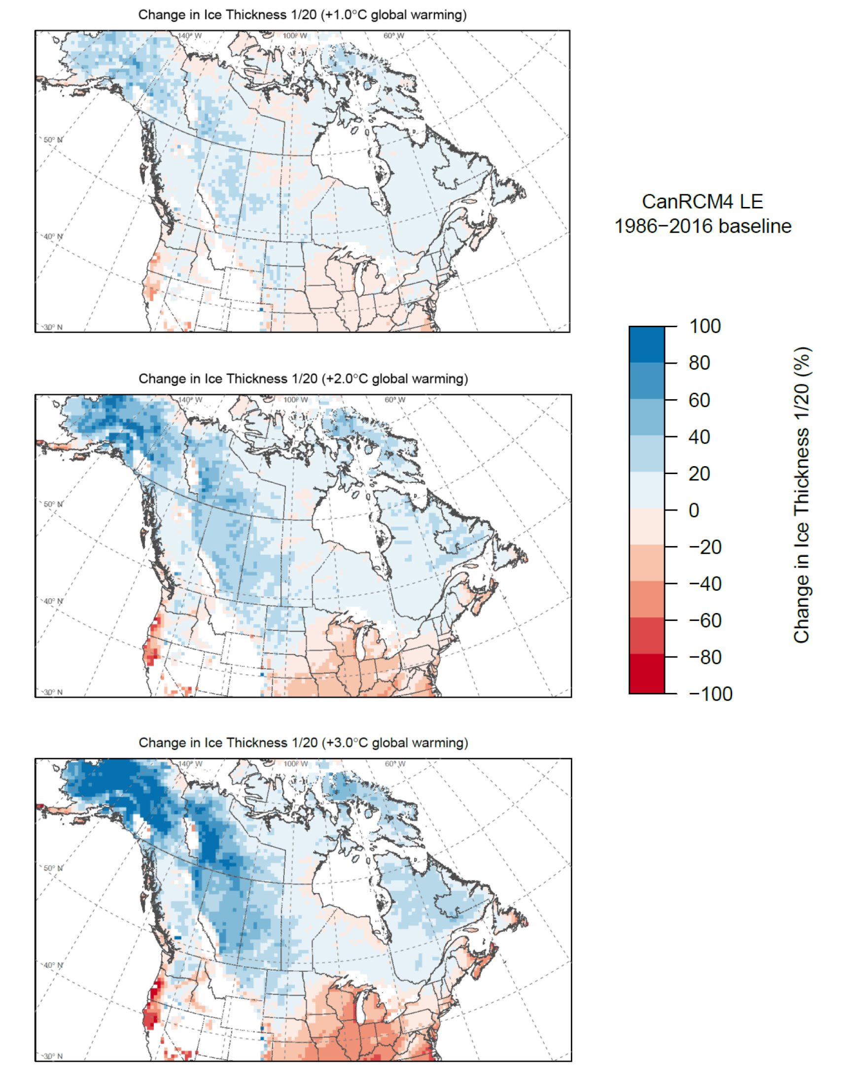
Table 6.2: CanRCM4 LE projected changes in design ice thickness for locations in Table C-2 in six Canadian regions and Canada as a whole for +1°C, +2°C, and +3°C global warming levels with respect to the 1986-2016 baseline period. Values represent the ensemble projection (25th percentile, 75th percentile) calculated from CanRCM4 LE.
| Change in ice thickness 1/20 [%] | Global warming level | ||
|---|---|---|---|
| Region | +1°C | +2°C | +3°C |
| British Columbia | 3.5 (-11.3, 19.5) | 3.1 (-14.1, 23.4) | 0.3 (-13.0, 14.8) |
| Prairies | 15.2 (-6.9, 40.0) | 27.6 (2.0, 58.9) | 38.1 (6.8, 73.2) |
| Ontario | 1.1 (-13.3, 17.5) | 0.3 (-16.7, 17.1) | -9.6 (-24.5, 9.2) |
| Quebec | 5.0 (-8.7, 20.7) | 9.3 (-4.6, 29.0) | 6.6 (-10.6, 27.8) |
| Atlantic | -4.4 (-20.5, 15.9) | -22.8 (-36.5, -1.0) | -39.5 (-52.0, -26.4) |
| North | 10.4 (-9.2, 47.9) | 21.0 (0.2, 59.3) | 33.0 (5.2, 79.0) |
| Canada | 3.4 (-11.5, 20.1) | 4.9 (-11.6, 23.6) | 2.0 (-14.9, 20.7) |
As changes in future extreme ice thickness are largely determined by changes in extreme freezing precipitation (Jeong et al., 2019)Reference 125, the spatial pattern of CanRCM4 LE projected changes to extreme freezing precipitation (Appendix 2.7) are similar to those for design ice accretion loads (Figure 6.4). Spatial patterns of projected changes to both extreme freezing precipitation and design ice loads are broadly consistent with the findings based on another Canadian RCM (CRCM5) simulation over Canada (Jeong et al., 2018)Reference 123.
CanRCM4 LE simulations of freezing precipitation and ice accretion exhibit large internal variability (see Table 6.2 and Figure 6.5). Emergence of the forced signal from the noise of internal variability only occurs in some regions at high global warming levels. Uncertainties other than those due to internal variability are not reflected in Table 6.2 and Figure 6.5. These include the choice of RCM and driving GCM, and choice of methods for calculating freezing precipitation and ice accretion. Model uncertainty, which affects both RCMs and their driving GCMs, likely stems from multiple factors including temperature and precipitation biases in the models, limitations in the representation of precipitation producing processes, differences between model and actual topography, and the fact that freezing rain and ice accretion processes are not represented explicitly.
Projected changes to design ice accretion loads in CanRCM4 LE are primarily driven by changes in the vertical temperature profile (Jeong et al., 2019)Reference 125, which directly affects the diagnosed frequency of freezing precipitation occurrence. Freezing precipitation typically occurs when upper level air temperatures that are high enough to cause melting (e.g., 850 hPa temperature T850 > 3°C) coincide with sub-freezing surface air temperatures (Ts) that cause freezing (e.g., -10°C < Ts < 0°C). Warming at both upper levels and the surface (Figure 6.6) leads to a decrease in the future frequency of temperature conditions favourable to the occurrence of freezing rain over the US and western and eastern coastal regions of Canada at the +2°C global warming level, but an overall increase in the frequency of such conditions over most other regions of Canada.
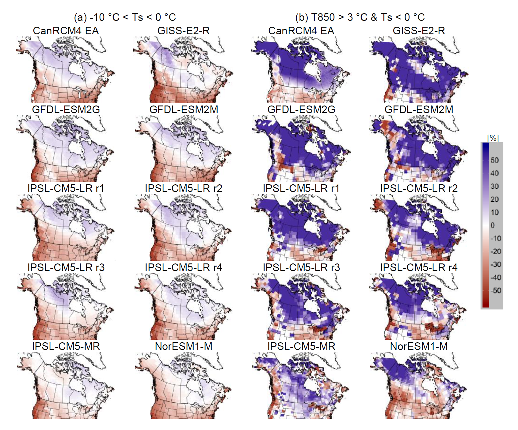
In order to provide an initial look at the effects of model uncertainty, CanRCM4 LE projected changes in conditions that favour freezing precipitation were compared with those projected by 9 CMIP5 GCMs (Figure 6.6) and found to be generally consistent. The GCMs, however, display some regional differences, particularly over northwestern coastal, northeastern, and central regions of Canada; 6 GCMs project decreases in the frequency of surface temperature between -10°C and approximately 0°C and associated frequency of favourable conditions for freezing precipitation occurrence over some regions in northwestern and/or northeastern Canada. Thus regional responses likely differ between models at the same global warming level, reflecting the presence of model uncertainty. Interpretation is further complicated by the large role of internal variability on projection uncertainty noted above and as can be seen by comparing results from individual simulations made with the same model. Also, interpretations are complicated by the fact that model temperature biases affecting surface and upper air temperatures will affect the frequency, intensity and spatial distribution of freezing precipitation in the current climate differently in every model, and thus the changes that are projected under warming. Because the production of freezing precipitation involves water phase changes that occur at a fixed temperature, simple temperature scaling considerations that seem to work well for precipitation generally are unlikely to be nearly as helpful in the case of freezing precipitation.
6.2.3 Interpretation
Ice accretion load is a Tier 3 variable. Projected changes at locations approximating Table C-2 locations are provided in Appendix 1.2. Values are based on projections from CanRCM4 LE. The spatial patterns of projected changes to freezing precipitation and ice accretion loads from the CanRCM4 LE are largely consistent with those projected by a different regional model (CRCM5), driven both by the same GCM and a different GCM over Canada (Jeong et al., 2018)Reference 123. This consistency provides some confidence that it would be reasonable to anticipate overall increases in future design ice accretion loads over most of Canada. The CanRCM4 LE, however, illustrates that the projections are subject to high internal variability, with forced changes having low signal-to-internal-noise ratios until global warming levels exceed +2°C. Values of the NS ratio are close to one at all levels of global warming. As discussed above, the projections are also almost certainly affected by model and algorithmic uncertainties that are, as yet, not quantified. There is medium confidence that ice accretion loads will increase over most of Canada as the climate continues to warm, but very low confidence in the CanRCM4 based projections of ice accretion load changes, including the details of spatial variations in the projected load changes.
It is not possible to assess the place and warming level specific load change projections provided in Appendix 1.2. Nevertheless, given the potential impact of catastrophic structural failure due to excess ice loads, a conservative approach that considers projected load increases in those locations where increases are projected and that uses loads established from recent historical data in all other locations would seem prudent.
6.3 Permafrost
6.3.1 Assessment
Permafrost is often defined as a subsurface material with temperature continuously lower than 0°C for two or more years. Buildings and infrastructure in permafrost affected areas commonly use near-surface permafrost as their solid foundations (Zhou et al., 2008)Reference 127. At present, permafrost is distributed across high-latitude regions, covering about half of Canada (Heginbottom, 1995)Reference 128 and 80% of Alaska (Jorgenson et al., 2008)Reference 129. Over northern North America, continuous permafrost is found almost everywhere in the area north of the boreal tree line, while discontinuous permafrost tends to be found south of the tree line (Brown et al., 1998Reference 130; see also Figure 6.7).
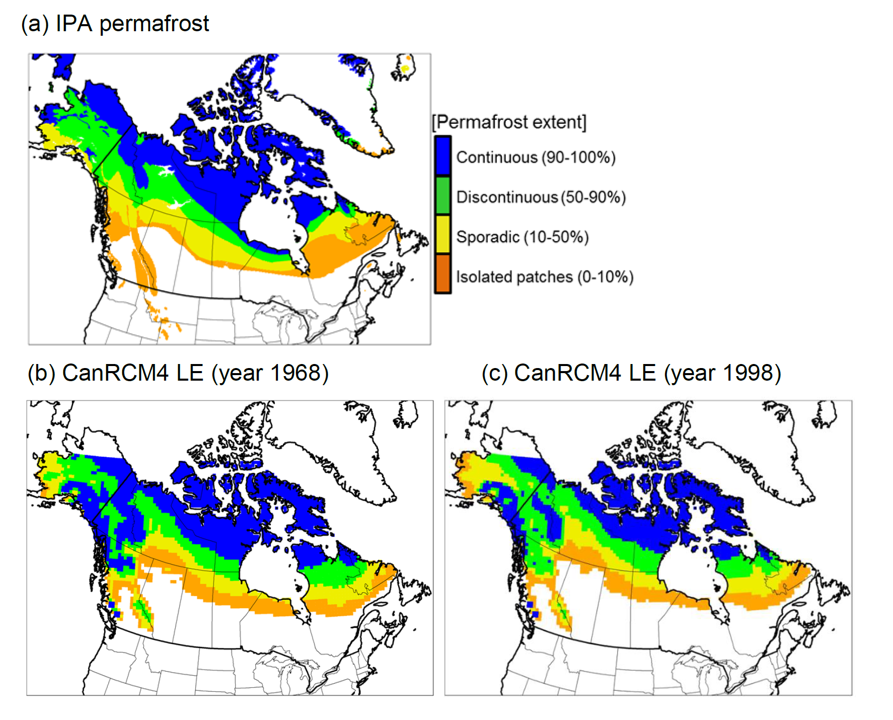
The CSA (2014)Reference 2 provides approximate southern boundaries of continuous and discontinuous (including sporadic and isolated patches) permafrost zones. The CSA (2014)Reference 2 permafrost zones were developed based on information obtained from Brown (1968)Reference 131 and ten different source maps from 1968 to 1988 (Heginbottom, 1995)Reference 128. Consequently, these maps do not reflect recent degradation of the marginal permafrost region over northern North America (e.g., Jorgenson et al., 2008Reference 129; Thibault and Payette, 2009Reference 132). Permafrost is known to be highly sensitive to warming (Wei et al., 2009Reference 133; Paquin and Sushama, 2015Reference 134). Permafrost degradation has been observed in northern North America (Jorgenson et al., 2006Reference 129; Fortier et al., 2007Reference 135; Thibault and Payette, 2009Reference 132).
Different approaches can be used to evaluate the potential impact of continued global warming on permafrost. One often used approach relies on projected changes in soil temperatures simulated by fully coupled atmosphere-ocean-land-sea ice GCMs (Sazonova and Romanovsky, 2003Reference 136; Zhang et al., 2008Reference 137; Koven et al., 2013Reference 138; Slater and Lawrence, 2013Reference 139). These studies indicate there is high confidence that future global warming will result in significant permafrost thawing in the regions studied. The magnitude of the projected change is, however, much less certain as there is wide variation in the present extent and projected future shrinkage of near-surface permafrost quantified directly from GCM soil temperatures. This is because results are highly dependent on the ability of GCMs to represent the near-surface climate and soil thermal regimes in cold climates (Koven et al., 2013)Reference 138. RCMs have some potential to reduce biases in soil temperatures of GCM simulations by improving spatial resolution and the representation of physical processes, but realizing this potential would require much more detailed information than currently utilized in such models to describe the spatial variations in soil and land surface properties (Paquin and Sushama, 2015)Reference 134.
Another approach is to employ indirect near-surface permafrost indices that are derived from surface climate valuables such as surface temperature and snow depth. The surface frost index (SFI) is an indirect approach that has been successfully used to evaluate the sustainability of near-surface permafrost under scenarios of climate change (Anisimov and Nelson, 1996Reference 140; Slater and Lawrence, 2013Reference 139; Guo and Wang, 2016Reference 141). This index is calculated from an estimate of the annual surface temperature cycle and monthly snow depths, which are required to account for the insulating effect of snow that sits on the land surface. The SFI index yields dimensionless values between zero and one that can be used to classify permafrost as isolated, sporadic, (extensive) discontinuous, or continuous permafrost based on thresholds suggested by Anisimov and Nelson (1996)Reference 140. Using such an approach Slater and Lawrence (2013)Reference 139 estimated that there would be around 1.67 ± 0.7 x 10⁶ km2 degradation of future near-surface permafrost extent per 1°C of global temperature increase from 19 CMIP5 GCMs under the RCP 8.5 scenario. This is consistent with IPCC (2013)Reference 4, who noted that the area of near-surface (e.g., within 3 m of the surface) permafrost could be reduced by between 37 to 81% by the end of the 21st century, depending on emission scenarios and associated increases in surface air temperature.
According to the CCCR (Bush and Lemmen, 2019)Reference 3, observations show increases in permafrost temperature (e.g., about 0.1°C per decade in the central Mackenzie Valley and 0.3 to 0.5°C per decade in the high Arctic (Alert) over the past 3-4 decades) and active layer thickness (approximately 10% since 2000 in the Mackenzie Valley) (high confidence), and widespread formation of thermokarst landforms across northern Canada (medium confidence). Projected increases in mean air temperature over land underlain with permafrost in all emissions scenarios are virtually certain to result in continued permafrost warming and thawing over large areas by mid-century, with impacts on northern infrastructure and the role of northern terrestrial ecosystems in the carbon cycle.
6.3.2 Targeted research
Given the level of uncertainty in direct simulation of permafrost extent in climate models, as well as the unavailability of archived soil temperature information from CanRCM4 LE, the simple SFI approach was used to produce CanRCM4 based projections of future permafrost extent. Compared to the International Permafrost Association (IPA) observations (Figure 6.7), CanRCM4 LE yields smaller near-surface permafrost extent during the comparable period (i.e., compare Figure 6.7a with Figure 6.7b and Figure 6.7c) when using the SFI approach, indicating that substantial biases are present relative to IPA even at the beginning of the period represented by the IPA map.
Based on the SFI approach, CanRCM4 LE projects substantial decreases in future near-surface permafrost extent over northern North America (Figure 6.8). The fractional reduction in permafrost affected area might be more robust than either the representation of the baseline extent (which is shown in grey), or the spatial details regarding transitions between permafrost types. Future permafrost degradation is highly dependent on increases in global mean temperature and the associated increases in regional surface temperature. CanRCM4 LE projects that future near-surface permafrost area over Canada (including all continuous and discontinuous regions) will decrease by around 16% per 1°C of global temperature increase (Figure 6.9). These results are comparable to the results of Guo and Wang (2016)Reference 141. They found 45% ± 10% and 68% ± 13% degradation of permafrost from the CMIP5 multi-model ensemble under the RCP4.5 and RCP8.5 scenarios, respectively, over Canada for the 2080-2099 period relative to the 1986-2005 period. Therefore, there is very high confidence in the future reduction of near-surface permafrost areas in Canada. Nevertheless, there is very low confidence in the magnitude of reduction of projected changes from CanRCM4 LE and in where and when transitions between continuous, discontinuous, sporadic and isolated patches permafrost zones will occur. A key reason for this low level of confidence is uncertainty in the simulation of the baseline permafrost distribution over Canada, which is affected by model biases, and limitations of the SFI approach that considers only surface climate information to diagnose near-surface permafrost status.
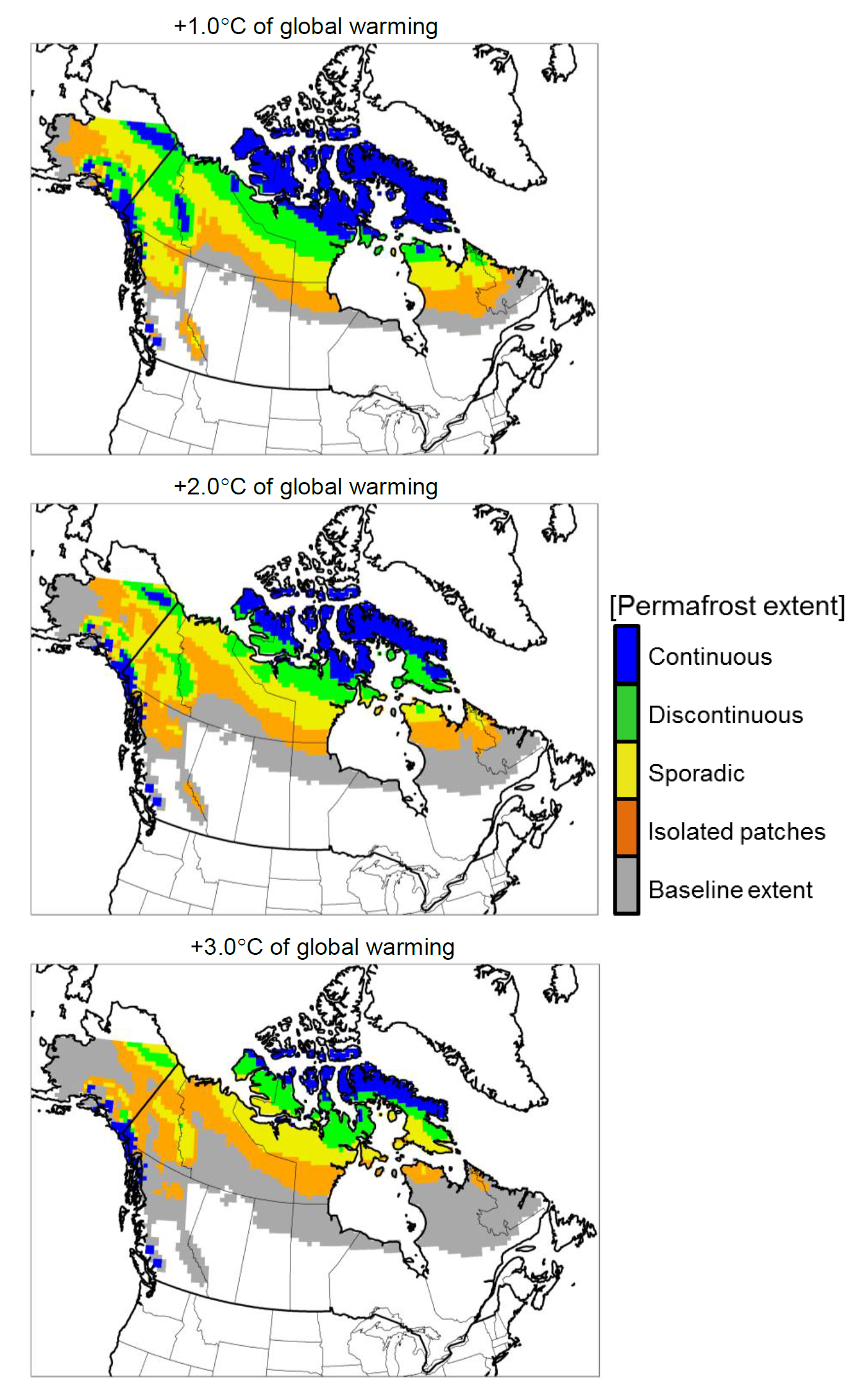
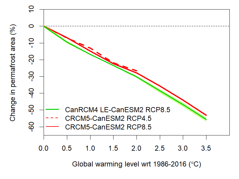
Projected relative changes to near-surface permafrost extent based on CRCM5 forced with the same GCM but under different emission scenarios (RCP4.5 and RCP8.5) are similar to each other and to CanRCM4 LE projected changes at the same global warming level (Figure 6.9). The effect of internal variability on relative changes in the permafrost affected area in the CanRCM4 is small (Figure 6.9), as would be expected for an index summarizing temperature dominated changes over a large area.
6.3.3 Interpretation
Permafrost is a Tier 3 variable. Given the links between reductions in near-surface permafrost extent and long-term surface warming trends, which are well understood, there is very high confidence in continued degradation of future near-surface permafrost extent over northern Canada at global warming levels higher than the baseline (Figure 6.8 and Figure 6.9). Projections of relative changes in the size of the area that is permafrost-affected from two Canadian RCMs – CanRCM4 LE and CRCM5 – agree and are consistent with findings from previous studies based on GCM projections.
There is, however, considerable uncertainty in the current permafrost distribution both in the IPA observations and climate model simulations, which affects projections of the location, type, and actual areal extent of future near-surface permafrost. Moreover, the indirect SFI approach is only capable of approximating the sustainability of near-surface permafrost, and can yield quite different results than those based on direct simulation of soil temperatures by climate models. Also, this approach requires the use of absolute temperature thresholds and snowfall amounts, and thus is sensitive to model biases. Very little, if any research, to determine the impacts of those biases on inferred permafrost location, type and extent has been performed to date. There is thus very low confidence in the future locations and areal extents of the different permafrost zones.
7. Summary and conclusions
This report has assessed projected future changes in B&CPI climatic design variables for Canada, based on published literature along with evidence that is directly available from the targeted research based on the CanESM2-CanRCM4 ensemble. Climatic design variables have been grouped into three tiers according to the assessed confidence in future projections for Canada as a whole:
Tier 1 variables are those for which there is generally high or very high confidence in the future projections for a given level of global warming. This level of confidence is afforded by in-depth understanding of the processes involved, as well as an abundant and a strong body of evidence (including evidence for other parts of the world) that deals with the causes of observed changes. This implies relatively high confidence in projected change factors for these variables, which suggests that specific values of these change factors could be considered when designing new infrastructure if justified from an engineering perspective and if suitable approaches exist to consider remaining uncertainties, including uncertainty in the amount of warming that might occur by the end of the service life of the structure that is being designed.
Tier 2 variables are those for which there is generally medium confidence in the future projections for a given level of global warming. In most instances, an assessment of medium confidence means there is some understanding of the processes that lead to future change. This might be supplemented by a body of evidence linking the causes of observed changes at large scales, but generally, such evidence would be much less extensive, with available studies showing a lower degree of consistency, than for Tier 1 variables. In contrast to situations when climate scientists have high or very high confidence, climate scientists are generally not able to estimate the likelihood of a projected change when they determine that they have medium confidence in future projections. Change factors for these variables are therefore more suitable for cost/benefit analyses or for a risk analysis, as well as for the exploration of uncertainty associated with design.
Tier 3 variables are those for which there is low or very low confidence in the future projections for a given level of global warming. Low or very low confidence is given to projections for variables that have not been widely studied in the published literature or for which the processes involved are poorly understood. In some instances, very low confidence is given to projections for variables that are diagnosed indirectly, for example, using empirical relationships because process understanding is limited. While change factors are projected, they are likely best suited to exploring the potential impacts of climate change on structural reliability in different warming and load combination scenarios.
7.1 Temperature
Climatic design variables related to surface temperature are Tier 1 variables. Available evidence from the CCCR (Bush and Lemmen, 2019)Reference 3 and climate model simulations suggest that it is virtually certain that Canada’s climate will warm further in the future. Projected increases in annual mean temperature in regions of Canada assessed in this report are about 1.5 to 2 times the corresponding increases in the global mean temperature, with larger increases in the North. Regional warming is a robust signal that emerges from the noise of historical climate variability at very low levels of global mean temperature change. Given the convergence of evidence from international and national assessments, there is high confidence in future projections of climatic design data related to surface temperature. Increases in January and July design temperatures and minimum and maximum mean daily temperatures and decreases in cold heating degree days will occur in all regions of Canada. Spatially, climatic design data that occur during the cold part of the year tend to increase more as one moves from south to north, whereas changes in hot extremes are more spatially uniform. In general, projected changes in temperature extremes are roughly proportional to changes in global mean temperature, with the constant of proportionality depending on variable, being equal to or exceeding that for annual mean temperature. Relative to projections of annual mean temperature, for which there is very high confidence, uncertainty for projections of temperature indices of extremes and other local temperature characteristics is larger due to higher internal variability, the influence of model bias on threshold exceedances, and higher uncertainty in climate model performance for extremes.
7.2 Precipitation and moisture
Annual precipitation and rainfall are Tier 2 variables. Evidence assessed in CCCR (Bush and Lemmen, 2019)Reference 3 and simulations from CanESM2-CanRCM4 LE suggests that there is high confidence that annual precipitation and rainfall will increase in Canada with global warming. Due to lower signal-to-noise ratio relative to temperature, as well as evidence that model uncertainty contributes more substantially to overall projection uncertainty, there is low to medium confidence in the projected percentage change in regional precipitation and rainfall. Projected increases in annual precipitation and rainfall are again roughly proportional to changes in global mean temperature, with greater rates of intensification in the North and, for rainfall, in mountainous regions in western Canada. In all regions, larger relative increases are projected for rain than total precipitation.
One day (50-year return period) and 15-min (10-year return period) rain are also Tier 2 variables. The CCCR (Bush and Lemmen, 2019)Reference 3 judged that it is likely that extreme precipitation will increase in Canada in the future, although the magnitude of the increase at regional scales is much more uncertain. At this time, it is recommended that projections of extreme one day and 15-min rain design data be made following the Clausius-Clapeyron (CC) relation, which suggests an intensification of ~7%/°C of local annual mean temperature change. This is supported by the fact that the intensification of extreme precipitation with warming over Canada in different climate models appears to be roughly consistent with the theoretical CC relationship. There is, however, some evidence that there may be deviations from this rate for different regions (higher along the coasts), accumulation durations (higher for shorter durations), and rarer events (higher for more rare events), albeit with very low to low confidence on such details. The scientific basis for so-called “super-CC scaling” with intensification substantially higher than the CC rate for short durations (6-hourly or less) remains unclear.
Annual mean relative humidity is a Tier 3 variable. According to IPCC (2007)Reference 72, globally “a broad-scale, quasi-unchanged [relative humidity] response [to climate change] is uncontroversial”. Overall, there is generally high confidence that future changes in relative humidity will be small. IPCC (2014)Reference 142 finds that “although the CMIP5 projected changes are small [there is] medium confidence that reductions in near-surface [relative humidity] over many land areas are likely.”
Consistent with international assessments, projections from CanESM2-CanRCM4 LE indicate little to no change in annual relative humidity over Canada. However, whereas CMIP5 GCMs project a small drying trend, CanRCM4 LE projects a small moistening trend. Given the small signal, relatively large uncertainty in multi-model assessments, and conflicting sign of change between CanRCM4 LE and CMIP3/CMIP5 GCMs, confidence in the magnitude of change over regions of Canada is very low.
7.3 Wind pressures
Design wind pressure is a Tier 3 variable. While there is some consistency amongst projections by different models that changes in future design wind pressures over Canada will be small, this is subject to considerable uncertainty due to the general inability of coarse resolution climate models to resolve many of the physical processes that drive extreme winds and low signal-to-noise ratio. Available literature and model projections indicate small increases in future design wind pressures over British Columbia, Ontario, and Atlantic regions at higher than +3°C global warming levels, but confidence in these projections is very low. Continuous monitoring of new research and assessments is warranted in those regions, and, more generally, across Canada.
Driving rain wind pressure (DRWP) is also a Tier 3 variable. While there is medium confidence that design DRWP will increase, confidence in the spatial pattern and magnitude of projected DRWP changes is very low due to the large uncertainty in wind extremes. Projected changes in temperature and precipitation, and hence rainfall, are relatively well understood over Canada, as compared to the changes in mean and extreme wind speeds. However, increases in future design wind pressure are projected over British Columbia, Ontario, and Atlantic regions at higher than +3°C global warming levels (very low confidence); hence, there is potential for additional increases in DRWP due to changes in the wind hazard in these regions.
7.4 Snow and ice
Snow load is a Tier 3 variable. There is medium confidence that snow loads will decrease over most of southern Canada. Projections from different models are consistent and the linkages between changes in temperature, precipitation, and snow water equivalent (SWE; the mass of the frozen water sitting on the land surface) are reasonably well understood at the spatial scales represented by the models.
There is, however, only low confidence in the magnitude of the decrease in the snow component of snow loads due to the role of internal variability as well as uncertainty due to the simplified snow models used in current regional climate models. Furthermore, greater uncertainty is expected in areas with complex terrain that are not well resolved by relatively coarse resolution climate models. In the North, where precipitation increases may offset reductions due to increasing temperatures, there is very low confidence that there will be either no change or a modest increase.
There is also very low confidence about future projections of the rain component of snow load, due in large part to high internal variability, as well as the compound nature of the variable – rain must occur coincident with the presence of snow on the ground.
Ice accretion load is a Tier 3 variable. Projections are undoubtedly affected by climate model and ice accretion estimation uncertainties that are, as yet, not quantified. Consequently, there is very low confidence in the CanRCM4 based projections of ice accretion load changes, including the details of spatial variations in the projected load changes and even the regional variation in the sign of the projected changes. Projections are subject to high internal variability, and hence the signal-to-noise ratio of the forced changes in CanRCM4 is low until global warming levels exceed +2°C. While spatial patterns of changes in upper level and surface temperature conditions favourable for freezing precipitation are broadly similar amongst members of a multi-model ensemble of climate models, regional differences under the same level of global warming are nevertheless substantial.
Permafrost is a Tier 3 variable. Nevertheless, given the strong links between reductions in permafrost extent and long-term surface warming trends, which are well understood, there is very high confidence in continued degradation of future near-surface permafrost extent over northern Canada. Projections are, however, preliminary and are based on a simple, indirect Surface Frost Index approach, rather than direct simulation of soil temperatures. There is thus considerable uncertainty and very low confidence in projections of future locations and areal extents of the different permafrost zones.
7.5 Conclusions and path forward
The projected changes for various regions and for specific B&CPI sites in this report are based on a large 50-member ensemble of the CanESM2-CanRCM4 climate modelling system. The proper interpretation of these data must take into consideration that this information is conditional on this specific set of simulations and on the level of scientific confidence that can be placed in the projections. The exact values in these projections would differ should a different set of model simulations be used. As the confidence in this report is assessed at the spatial scale of Canada’s land mass, and as confidence generally decreases with the decrease of spatial scale because of reduction in signal-to-noise ratio, confidence in the regional and local/site specific projections is lower. Confidence is also lower for projections of changes in the magnitude of a particular climatic load than for projections of its direction of change.
The rapid development of climate science and technology should, in practice, lead to better process understanding and improved climate modelling capacity, for example through the development and application of higher resolution GCMs and RCMs with improved process representation and the production of ensemble simulations with very high-resolution convection-permitting RCMs. In the case of regional climate modelling experiments, a critical challenge is to design and obtain modelling centre participation in experiments that effectively sample model uncertainty, across both GCMs and RCMs. This is critical in order to better understand which projected design value changes are robust and insensitive to the choice of GCM-RCM combination, and which other projected changes remain strongly affected by such sources of uncertainty. Note also that while there is rapidly increasing interest and research activity using convection-permitting models, these models remain extraordinarily expensive to use, have many of their own caveats and remain dependent on a range of parameterizations despite their very high resolution. As research with these models becomes more mature, it will be possible to make informed judgements about which aspects of convection-permitting simulations of changes in design data are robust. More generally, process understanding still holds the key towards making more robust projections of extreme precipitation, relative humidity, wind pressures, snow and ice loads, and permafrost (Tier 2 and 3 variables). Gaining the physical process understanding necessary to make credible regional projections, with improved confidence, requires significant, targeted basic climate science research. Improvements in climate modelling and process understanding will ultimately lead to better climate change assessments for B&CPI and projections of climatic design data in Canada. This in turn will facilitate the development of more robust quantitative guidance and commentary in new editions of the National Building Code of Canada (NBCC Table C-2) and the Canadian Highway Bridge Design Code (CHBDC CSA S6 Annex A3.1).
9. Appendices
Appendix 1
Appendix 1.1: Timing of global warming
Timing of global warming. Year at which the indicated global mean ΔT relative to 1986-2016 reference period is irrevocably exceeded by the specified multi-model statistic. CMIP5one = single ensemble member per model; CMIP5all = Models with > 1 ensemble member averaged before constructing that model’s mean. Ensemble mean ΔT smoothed using a 31-year moving window with exceedance test conducted on central value.
| Scenario | Nruns | ΔT = 0.5°C | 1.0 | 1.5 | 2.0 | 2.5 | 3.0 | 3.5 | 4.0 |
|---|---|---|---|---|---|---|---|---|---|
| Year of exceedance: multi-model mean (upper, CMIP5one; lower, CMIP5all) | |||||||||
| RCP2.6 | 32 | 2023 | − | − | − | − | − | − | − |
| 65 | 2023 | − | − | − | − | − | − | − | |
| RCP4.5 | 42 | 2022 | 2043 | 2071 | − | − | − | − | − |
| 108 | 2022 | 2043 | 2071 | − | − | − | − | − | |
| RCP6.0 | 25 | 2025 | 2049 | 2069 | 2087 | − | − | − | − |
| 47 | 2025 | 2049 | 2069 | 2088 | − | − | − | − | |
| RCP8.5 | 39 | 2020 | 2035 | 2047 | 2059 | 2069 | 2080 | 2090 | 2100* |
| 81 | 2020 | 2035 | 2048 | 2059 | 2069 | 2080 | 2091 | 2100* | |
| Scenario | Nruns | ΔT = 0.5°C | 1.0 | 1.5 | 2.0 | 2.5 | 3.0 | 3.5 | 4.0 |
|---|---|---|---|---|---|---|---|---|---|
| Year of exceedance: multi-model median (upper, CMIP5one; lower, CMIP5all) | |||||||||
| RCP2.6 | 32 | 2025 | − | − | − | − | − | − | − |
| 65 | 2025 | − | − | − | − | − | − | − | |
| RCP4.5 | 42 | 2023 | 2044 | 2078 | − | − | − | − | − |
| 108 | 2023 | 2044 | 2078 | − | − | − | − | − | |
| RCP6.0 | 25 | 2026 | 2052 | 2072 | 2098 | − | − | − | − |
| 47 | 2026 | 2052 | 2072 | 2098 | − | − | − | − | |
| RCP8.5 | 39 | 2021 | 2036 | 2050 | 2060 | 2072 | 2082 | 2092 | − |
| 81 | 2021 | 2036 | 2050 | 2060 | 2072 | 2082 | 2092 | − | |
| Scenario | Nruns | ΔT = 0.5°C | 1.0 | 1.5 | 2.0 | 2.5 | 3.0 | 3.5 | 4.0 |
|---|---|---|---|---|---|---|---|---|---|
| Year of exceedance: multi-model upper quartile (upper, CMIP5one; lower, CMIP5all) | |||||||||
| RCP2.6 | 32 | 2020 | 2100 | − | − | − | − | − | − |
| 65 | 2020 | 2100 | − | − | − | − | − | − | |
| RCP4.5 | 42 | 2020 | 2036 | 2057 | 2079 | − | − | − | − |
| 108 | 2020 | 2036 | 2057 | 2079 | − | − | − | − | |
| RCP6.0 | 25 | 2020 | 2042 | 2062 | 2079 | 2095 | − | − | − |
| 47 | 2020 | 2042 | 2062 | 2079 | 2095 | − | − | − | |
| RCP8.5 | 39 | 2017 | 2033 | 2043 | 2052 | 2062 | 2071 | 2079 | 2089 |
| 81 | 2017 | 2033 | 2043 | 2052 | 2062 | 2071 | 2079 | 2089 | |
- Source of CMIP5 temperature output is the KNMI Climate Explorer, https://climexp.knmi.nl/start.cgi.
- Near endpoints, 31-year moving window shrinks to n-year symmetric window with n approaching 1 at endpoint.
- No entry (−) means specified model statistic does not exceed the specified ΔT before 2100.
Appendix 1.2: Projected changes
Projected changes for climatic variables at locations approximating those included in Table C-2 of NBCC are provided in the linked Excel spreadsheets. Refer to chapter 2, chapter 3, chapter 4, chapter 5 and chapter 6 for the discussion of methodology, assessed levels of confidence, and guidance for each variable.
Values provided in the +##C [+0.5C to +3.5C] sheets are projected future changes in climate design data for the specified levels of global mean temperature change (see section 2.5.1 and Appendix 1.1). In general, changes are obtained from projections at the closest CanRCM4 LE land grid cell. Projected changes for Rn15m and Rn1Day are based on Clausius-Clapeyron scaling (7% per °C) of annual mean temperature change (AnnTmean); values of NS ratio for these variables are based on ensemble spread from extreme value analyses of raw 1-hr and one day annual maxima from CanRCM4 LE, respectively.
Importantly, tabulated values for a given climatic design variable are based on projections of change that have been assessed for the regional-to-national scale at a given level of confidence based on supporting evidence and process understanding. The specific values at individual locations should be considered to have lower confidence.
Values at individual locations are coloured according to ranges of the noise-to-signal (NS) ratio as determined from CanRCM4 LE projections and ensemble spread:

Assessed levels of confidence are indicated by the following labels:
- Tier 1 variables (high or very high confidence)
- Tier 2 variables (medium confidence)
- Tier 3 variables (very low or low confidence)
Changes are expressed in the units given below:
| Appendix1.2_+##C_CHBDC.xls | |
|---|---|
| Variable | Tier |
| iceThickFootnote 11xi – Ice thickness (1/20) [%] | Tier 3 (very low or low confidence) |
| maxTmean - Maximum mean daily air temperatures [°C] | Tier 1 (high or very high confidence) |
| minTmean - Minimum mean daily air temperatures [°C] | Tier 1 (high or very high confidence) |
| Q10 - Hourly wind pressures (1/10) [%] | Tier 3 (very low or low confidence) |
| Q25 - Hourly wind pressures (1/25) [%] | Tier 3 (very low or low confidence) |
| Q50 - Hourly wind pressures (1/50) [%] | Tier 3 (very low or low confidence) |
| Q100 - Hourly wind pressures (1/100) [%] | Tier 3 (very low or low confidence) |
|
Download Appendix 1.2 CHBDC data: |
|
| Appendix1.2_+##C_NBCC.xls | |
|---|---|
| Variable | Tier |
| AnnP - Annual total precipitation [%] | Tier 2 (medium confidence) |
| AnnR - Annual rain [%] | Tier 2 (medium confidence) |
| AnnTmean - Annual mean air temperature [°C] | Tier 1 (high or very high confidence) |
| DRQ - Driving rain wind pressure [%] | Tier 3 (very low or low confidence) |
| HDD - Degree days below 18°C [°C days] | Tier 1 (high or very high confidence) |
| RH - Relative humidity [%] | Tier 3 (very low or low confidence) |
| Q10 - Hourly wind pressures (1/10) [%] | Tier 3 (very low or low confidence) |
| Q50 - Hourly wind pressures (1/50) [%] | Tier 3 (very low or low confidence) |
| Rn15m - 15-min rain (1/10) [%] | Tier 2 (medium confidence) |
| Rn1Day - One day rain (1/50) [%] | Tier 2 (medium confidence) |
| SLr - Rain load (1/50) [%] | Tier 3 (very low or low confidence) |
| SLs - Snow load (1/50) [%] | Tier 3 (very low or low confidence) |
| TJan10 - Design Temperatures January 1% [°C] | Tier 1 (high or very high confidence) |
| TJan25 - Design Temperatures January 2.5% [°C] | Tier 1 (high or very high confidence) |
| TJuly - Design Temperatures July 2.5% dry [°C] | Tier 1 (high or very high confidence) |
| TwJuly - Design Temperatures July 2.5% wet [°C] | Tier 1 (high or very high confidence) |
|
Download Appendix 1.2 NBCC data: |
|
Appendix 2: Links to published papers
Appendix 2.1
Arora, V.K. and A.J. Cannon, 2018. A brief background on climate models: the source of future climate information. In: P. Mukhopadhyaya (ed.), 1st International Conference on New Horizons in Green Civil Engineering (NHICE-01), Victoria, BC, Canada, April 25-27, 2018. ISBN: 978-1-55058-620-6. p. 348-356 https://onlineacademiccommunity.uvic.ca/nhice/wp-content/uploads/sites/2382/2019/02/Proceedings_22Feb2019.pdf
Appendix 2.2
Scinocca, J. F., Kharin, V. V., Jiao, Y., Qian, M. W., Lazare, M., Solheim, L., ... & Dugas, B. (2016). Coordinated global and regional climate modeling. Journal of Climate, 29(1), 17-35. https://doi.org/10.1175/JCLI-D-15-0161.1
Appendix 2.3
Li, G., X. Zhang, A.J. Cannon, T.Q. Murdock, S. Sobie, F.W. Zwiers, K. Anderson, and B. Qian, 2018. Indices of Canada's future climate for general and agricultural adaptation applications. Climatic Change, 148(1-2):249-263. https://doi.org/10.1007/s10584-018-2199-x
Appendix 2.4
Li, C., F. Zwiers, X. Zhang, and G. Li, 2019. How much information is required to well constrain local estimates of future precipitation extremes? Earth’s Future, 7, 11-24. https://doi.org/10.1029/2018EF001001
Appendix 2.5
Zhang, X., F.W. Zwiers, G. Li, H. Wan, and A.J. Cannon, 2017. Complexity in estimating past and future extreme short-duration rainfall. Nature Geoscience, 10:255-259. https://doi.org/10.1038/NGEO2911
Appendix 2.6
Cannon, A.J. and S. Innocenti, 2019. Projected intensification of sub-daily and daily rainfall extremes in convection-permitting climate model simulations over North America: Implications for future intensity-duration-frequency curves. Natural Hazards and Earth System Sciences, 19:421-440. https://doi.org/10.5194/nhess-19-421-2019
Appendix 2.7
Jeong, D.I., A.J. Cannon, and X. Zhang, 2019. Projected changes to extreme freezing precipitation and design ice loads over North America based on a large ensemble of Canadian regional climate model simulations. Natural Hazards and Earth System Sciences, 19:857-872. https://doi.org/10.5194/nhess-19-857-2019
10. List of acronyms
| List of acronyms | |
|---|---|
| B&CPI | Buildings and Core Public Infrastructure |
| CanAM4 | Canadian (CCCma) Atmospheric Model version 4 |
| CanESM2 | Canadian (CCCma) Earth System Model version 2 |
| CanRCM4 | Canadian (CCCma) Regional Climate Model version 4 |
| CC | Clausius-Clapeyron |
| CCCma | Canadian Centre for Climate Modelling and Analysis |
| CHBDC | Canadian Highway Bridge Design Code |
| CLASS | Canadian Land Surface Scheme |
| CoV | Coefficient of Variation, the ratio of standard deviation to the mean of a time series of annual maxima |
| CGCM3 | Canadian Global Climate Model version 3 |
| CMIP | Coupled Model Intercomparison Project (phase 3, CMIP3; and phase 5, CMIP5) |
| CORDEX | Coordinated Regional Downscaling Experiment |
| CRCM5 | Canadian Regional Climate Model version 5 |
| CRD | Climate Research Division |
| DRWP | Driving Rain Wind Pressure |
| ECCC | Environment and Climate Change Canada |
| ESM | Earth System Model |
| FP | Freezing Precipitation |
| GEM | Global Environmental Multiscale Model |
| GCM | Global Climate Model |
| GHG | Greenhouse Gas |
| HRCONUS | High-resolution Contiguous United States |
| IDF | Intensity-Duration-Frequency |
| IPA | International Permafrost Association |
| IPCC | Intergovernmental Panel on Climate Change |
| LE | Large Ensemble |
| NARCCAP | North American Climate Change Assessment Program |
| NBCC | National Building Code of Canada |
| NRC | National Research Council |
| PCIC | Pacific Climate Impacts Consortium |
| RCM | Regional Climate Model |
| NS ratio | noise-to-signal ratio, a measure of ensemble spread divided by the magnitude of projected change |
| RCP | Representative Concentration Pathway |
| SCE | Area of Snow Covered Extent |
| SFI | Surface Frost Index |
| SRES | Special Report on Emissions Scenarios |
| SWE | Snow Water Equivalent |
| Ts | Near-surface Air Temperature |
| T850 | Air Temperature at 850 hPa |
| WRF | Weather Research and Forecasting Model |